Gradient Boosting Regression Tree

Pseudo code

Input : Data ${x_{i}, y_{i}}_{i = 1}^{n}$ , and a differentiable Loss function $L (y_{i}, F (x))$
Step 1 : Initialized model with a constant value: $F_{0} (x) = \arg min_{γ} \sum_{i = 1}^{n} L (y_{i}, γ)$
Step 2 : for $m = 1$ to M:
(A) Compute $r_{i m} = - [\frac{\partial L (y_{i}, F (x_{i}))}{\partial F_{(} x_{i})}]_{F (x) = F_{m - 1} (x)}$ for $i = 1, . . . n$
(B) Fit a regression tree to the $r_{i m}$ values and create terminal regions $R_{i m}$ , for $j = 1, . . ., J_{m}$
(C) For $j = 1, . . ., j_{m}$ compute $r_{j m} = \arg min_{γ} \sum_{x_{i} \in R_{i j}} L (y_{i}, F_{m - 1} (x_{i}) + γ)$
(D) Update $F_{m} (x) = F_{m - 1} (x) + ν \sum_{j = 1}^{J_{m}} γ_{m} I (x \in R_{j m})$
Step 3 : Output $F_{M} (x)$

Details

Input : Data ${x_{i}, y_{i}}_{i = 1}^{n}$ , and a differentiable Loss function $L (y_{i}, F (x))$

미분 가능한 loss function으로 GBM에서는 L2 norm을 선택한다. 이 때 $\frac{1}{2}$ 는 계산상의 편의를 위해서 scaling constant이다.
Loss function : $L (y_{i}, F (x)) = \frac{1}{2} \sum_{i = 1}^{n} (y_{i} - F (x))^{2}$

loss <- function(y, yhat){
                return(mean(1/2*(y-yhat)^2))
}

Step 1 : Initialized model with a constant value: $F_{0} (x) = \arg min_{γ} \sum_{i = 1}^{n} L (y_{i}, γ)$

$\begin{aligned} F_{0} (x) & = \arg min_{γ} \sum_{i = 1}^{n} L (y_{i}, γ) \\ = \frac{d}{d γ} \frac{1}{2} \sum_{i = 1}^{n} (y_{i} - γ^{2}) \\ = - \sum_{i = 1}^{n} (y_{i} - γ) \\ = 0 \\ \Leftrightarrow \hat{γ} = \bar{y} \end{aligned}$

초기값은 y의 평균으로 계산한다.

1. Compute $r_{i m} = - [\frac{\partial L (y_{i}, F (x_{i}))}{\partial F_{(} x_{i})}]_{F (x) = F_{m - 1} (x)}$ for $i = 1, . . . n$
$\begin{aligned} r_{i m} & = - [\frac{\partial L (y_{i}, F (x_{i}))}{\partial F_{(} x_{i})}]_{F (x) = F_{m - 1} (x)}, i = 1, . . . n, m = # t r e e \\ \Leftrightarrow r_{i m} = y_{i} - F_{m - 1} (x_{i}) \end{aligned}$

$r_{i m}$ 은 negative gradient or pseudo residual이라고 한다. GBM은 residual을 기반으로 regression tree를 생성하는데 이 때 이용되는 residual 값이 $r_{i m}$ 으로 계산된 pseudo residual이다.

negative_residual <- function(y, yhat) {
                return(y - yhat)
}

1. Fit a regression tree to the $r_{i m}$ values and create terminal regions $R_{i m}$ , for $j = 1, . . ., J_{m}$
tree의 깊이는 보통 8~32 정도로 구성된다. full tree가 아닌 weak learner or weak tree를 만들기 때문에 tree의 terminal regions $R_{i m}$ 에는 여러 개의 값이 존재할 수 있다.
1. For $j = 1, . . ., j_{m}$ compute $r_{j m} = \arg min_{γ} \sum_{x_{i} \in R_{i j}} L (y_{i}, F_{m - 1} (x_{i}) + γ)$
이 때 tree의 terminal regions $R_{i m}$ 에 존재하는 여러 개의 값은 $r_{j m}$ : terminal region의 평균으로 계산된다.

$\begin{aligned} r_{j m} & = \arg min_{γ} \sum_{x_{i} \in R_{i j}} L (y_{i}, F_{m - 1} (x_{i}) + γ) \\ = \arg min_{γ} \sum_{x_{i} \in R_{i j}} \frac{1}{2} (y_{i} - (F_{m - 1} (x_{i}) + γ)) \\ \Leftrightarrow - \sum_{x_{i} \in R_{i j}} (y_{i} - F_{m - 1} (x_{i}) - γ)) = 0 \\ \Leftrightarrow \hat{γ} := t e r m i n a l r e g i o n 의 평 균 \end{aligned}$

1. Update $F_{m} (x) = F_{m - 1} (x) + ν \sum_{j = 1}^{J_{m}} γ_{m} I (x \in R_{j m})$

완성된 tree는 $\sum_{j = 1}^{J_{m}} γ_{m} I (x \in R_{j m})$ 로 표현되며 learning rate $ν$ 를 이용해서 예측값에 대한 개별 tree의 영향력을 조절한다. $ν$ 가 작으면 개별 tree의 영향력이 줄어들고, 계산량이 많아지지만 accuracy는 향상된다. $ν$ 가 크면 개별 tree의 영향력이 커지고, 계산량이 상대적으로 적으며, accuracy가 상대적으로 줄어든다.

Full code

구글 서치 중에 OLS 기반으로 gradient boosting 수행하는 코드를 발견했는데 gradient boosting 알고리즘을 이해하는데 많은 도움이 되었다(실제 패키지에서는 regression tree 기반으로 계산되기 때문에 theta 값은 계산되지 않는다)

grad_boost <- function(formula, data, nu = 0.01, stop, 
                       grad.fun, loss.fun, yhat.init = 0) {
  
  data <- as.data.frame(data)
  formula <- terms.formula(formula)
  X <- model.matrix(formula, data)
  
  y <- data[, as.character(formula)[2]] # as.character(formula)[2] : formula y~.에서 y에 해당하는 명칭

  fit <- yhat.init
  
  u <- grad.fun(y = y, yhat = fit) # pseudo residual 계산 
  
  theta <- rep(0, ncol(X))
  
  loss <- c()
 
  for (i in 1:stop) {
    
    # Design matrix를 이용한 regression, OLS 기반, Tree X 
    base_prod <- lm.fit(x = X, y = u) 
    theta_i <- coef(base_prod)
    
    # theta 값 업데이트 
    theta <- theta + nu*as.vector(theta_i)
    
    # yhat 값 업데이트
    fit <- fit + nu * fitted(base_prod)
    
    # pseudo residual 계산
    u <- grad.fun(y = y, yhat = fit)
    
    # loss 값 업데이트 
    loss <- append(loss, loss.fun(y = y, yhat = fit))
  }  
  names(theta) <- colnames(X)
  return(list(theta = theta, u = u, fit = fit, loss = loss, 
              formula = formula, data = data))
}

fit <- grad_boost(formula = Sepal.Length~Sepal.Width + Petal.Length + Petal.Width + Species, data = iris, stop = 1000, grad.fun = negative_residual, loss.fun = loss)
fit$theta

      (Intercept)       Sepal.Width      Petal.Length       Petal.Width 
        2.1711726         0.4958675         0.8292081        -0.3151416 
Speciesversicolor  Speciesvirginica 
       -0.7235307        -1.0234536

Using GBM package

패키지는 Tree 기반으로 계산되므로 고정된 coefficient 결과를 산출하지 않는다.
대신에 feature importance 값으로 변수별 상대적인 영향력을 볼 수 있다.

n.trees : tree의 갯수(the number of gradient boosting iteration), pseudo code에서 $M$ 에 해당
interaction.depth : tree당 최대 노드의 개수, 보통 8~32
shringkage : learning rate( $ν$ )
n.minobsinnode : terminal nodes의 최소 관찰값의 수
bag.fraction (Subsampling fraction) : training set을 나눌 비율. 기본적으로 stochastic gradient boosting 전략 채택. default : 0.5
train.fraction : 첫 train.fraction * nrows(data) 관찰값은 gbm fitting에 사용되고 나머지는 loss function에서의 out-of-sample 추정량을 계산하는데 사용됨. default = 1
cv.folds : cross validation fold의 개수
verbose : 모델 진행 상황을 모니터링할건지 유무
distribution : 분류 문제일 경우 - bernoulli, multinomial, regression 문제일 경우 - gaussian or tdist

보통 bag.fraction, train.fraction은 따로 지정하지 않음.

R code

library(gbm)
fit_pack <- gbm(formula = Sepal.Length~Sepal.Width + Petal.Length + Petal.Width + Species, 
                data = iris, 
                verbose = T, 
                shrinkage = 0.01, 
                distribution = 'gaussian')

Iter   TrainDeviance   ValidDeviance   StepSize   Improve
     1        0.6726             nan     0.0100    0.0076
     2        0.6650             nan     0.0100    0.0081
     3        0.6573             nan     0.0100    0.0080
     4        0.6493             nan     0.0100    0.0075
     5        0.6414             nan     0.0100    0.0073
     6        0.6326             nan     0.0100    0.0068
     7        0.6248             nan     0.0100    0.0072
     8        0.6171             nan     0.0100    0.0067
     9        0.6102             nan     0.0100    0.0068
    10        0.6028             nan     0.0100    0.0070
    20        0.5403             nan     0.0100    0.0058
    40        0.4424             nan     0.0100    0.0039
    60        0.3720             nan     0.0100    0.0030
    80        0.3182             nan     0.0100    0.0016
   100        0.2757             nan     0.0100    0.0014

summary(fit_pack)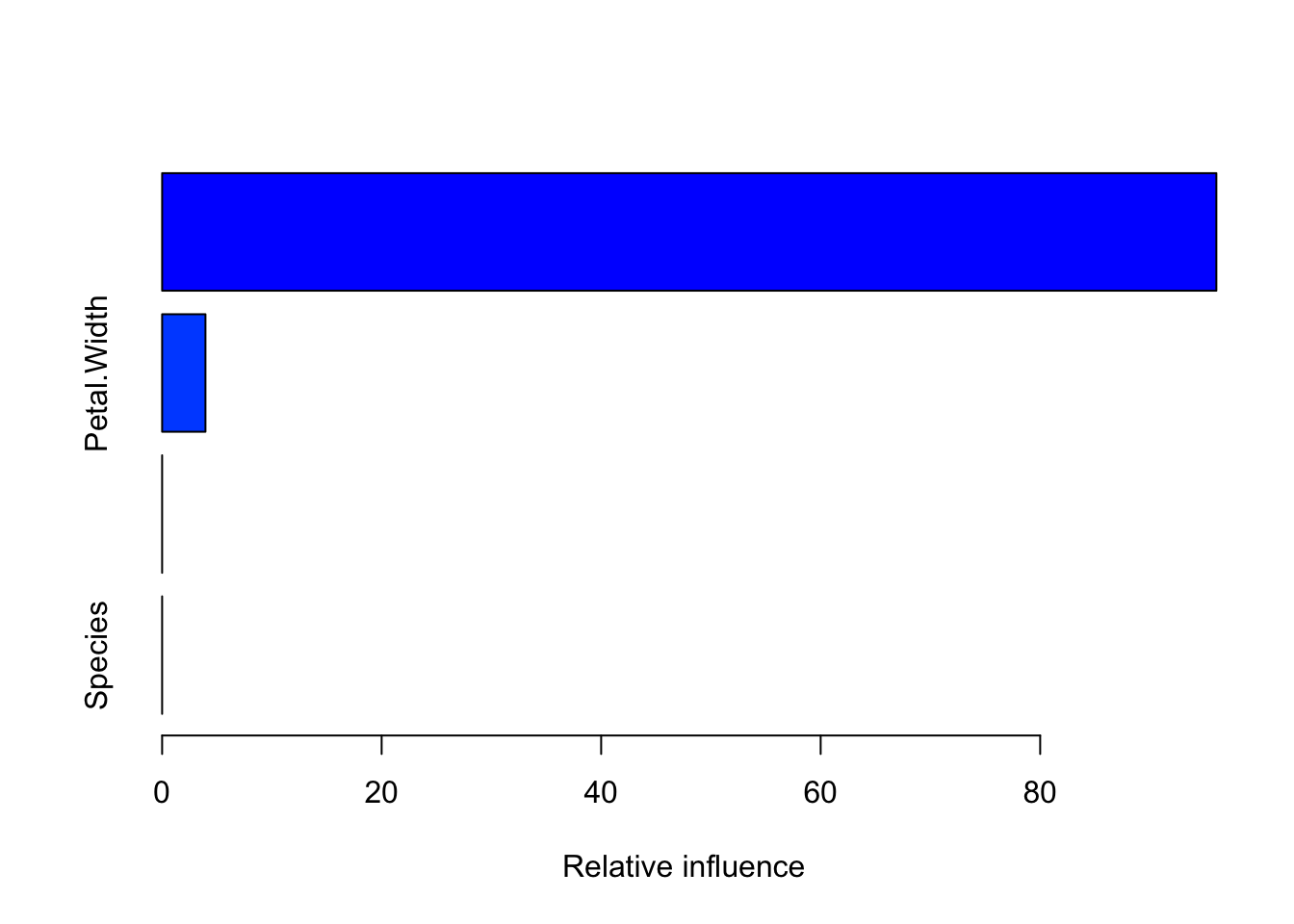

                      var rel.inf
Petal.Length Petal.Length 96.0517
Petal.Width   Petal.Width  3.9483
Sepal.Width   Sepal.Width  0.0000
Species           Species  0.0000

pretty.gbm.tree(fit_pack, i = 1)

  SplitVar SplitCodePred LeftNode RightNode MissingNode ErrorReduction Weight
0        1  4.5500000000        1         2           3       35.36091     75
1       -1 -0.0054100775       -1        -1          -1        0.00000     43
2       -1  0.0084729167       -1        -1          -1        0.00000     32
3       -1  0.0005133333       -1        -1          -1        0.00000     75
     Prediction
0  0.0005133333
1 -0.0054100775
2  0.0084729167
3  0.0005133333

pretty.gbm.tree()를 이용하면 개별 tree를 적합할 때 진행상황을 모니터링할 수 있다. 여기서의 predict 값은 개별 tree에 대한 값이므로 pseudo residual 값에 해당한다(참고 3).

참고 자료

참고 1 : https://www.youtube.com/watch?v=2xudPOBz-vs&list=PLblh5JKOoLUJjeXUvUE0maghNuY2_5fY6&index=2

참고 2 : https://medium.com/@statworx_blog/coding-gradient-boosted-machines-in-100-lines-of-code-d06b1d7bc084

참고 3 : https://stats.stackexchange.com/questions/237582/interpretation-of-gbm-single-tree-prediction-in-pretty-gbm-tree

Citation

BibTeX citation:

@online{don2021,
  author = {Don, Don and Don, Don},
  title = {Gradient Boosting Machine Tutorial},
  date = {2021-01-06},
  url = {https://dondonkim.netlify.app/posts/2021-06-12-gradient-boosting-regression/gbm.html},
  langid = {en}
}

For attribution, please cite this work as:

Don, Don, and Don Don. 2021. “Gradient Boosting Machine Tutorial.” January 6, 2021. https://dondonkim.netlify.app/posts/2021-06-12-gradient-boosting-regression/gbm.html.