tidymodels tutorial

tidymodels에 대한 간단한 소개

Author

Don Don

Published

March 6, 2021

tidymodels tutorial

tidymodels는 R 유저라면 한번쯤 써봤을 패키지인 tidyverse와 결이 같은 패키지이다. tidyverse가 데이터 전처리, 시각화를 간결한 파이프라인으로 만들 수 있는 것과 마찬가지로, tidymodels는 데이터 모델링 관점에서의 데이터 전처리, 모델링, 시각화 등을 쉽게 할 수 있게 고안된 패키지이다. tidyverse 수준으로 굉장히 완성도가 있고, R을 좋아하는 진성 유저들이 기존에 존재하는 패키지를 tidymodels와 결합하거나 새로운 함수를 끊임없이 만들고 있는 중이다.

tidymodels 설치 방법

tidymodels는 cran에 정식 등록된 패키지이므로 install_packages()로 설치가 가능하다. 설치 오류가 가끔 있는데 r 패키지를 전부 최신 버전으로 업데이트하면 오류 없이 설치가 가능하다.

tidymodels 패키지에는 예제 데이터로 ames 데이터가 내장되어있다. 간결한 설명을 위해 예제 데이터를 이용한다.

data(ames)
ames <- ames %>% janitor::clean_names()
head(ames)
# A tibble: 6 × 74
  ms_sub_class            ms_zoning lot_frontage lot_area street alley lot_shape
  <fct>                   <fct>            <dbl>    <int> <fct>  <fct> <fct>    
1 One_Story_1946_and_New… Resident…          141    31770 Pave   No_A… Slightly…
2 One_Story_1946_and_New… Resident…           80    11622 Pave   No_A… Regular  
3 One_Story_1946_and_New… Resident…           81    14267 Pave   No_A… Slightly…
4 One_Story_1946_and_New… Resident…           93    11160 Pave   No_A… Regular  
5 Two_Story_1946_and_New… Resident…           74    13830 Pave   No_A… Slightly…
6 Two_Story_1946_and_New… Resident…           78     9978 Pave   No_A… Slightly…
# … with 67 more variables: land_contour <fct>, utilities <fct>,
#   lot_config <fct>, land_slope <fct>, neighborhood <fct>, condition_1 <fct>,
#   condition_2 <fct>, bldg_type <fct>, house_style <fct>, overall_cond <fct>,
#   year_built <int>, year_remod_add <int>, roof_style <fct>, roof_matl <fct>,
#   exterior_1st <fct>, exterior_2nd <fct>, mas_vnr_type <fct>,
#   mas_vnr_area <dbl>, exter_cond <fct>, foundation <fct>, bsmt_cond <fct>,
#   bsmt_exposure <fct>, bsmt_fin_type_1 <fct>, bsmt_fin_sf_1 <dbl>, …

Data split

데이터 모델링을 진행할 때 홀드 아웃 방식으로 train set과 test set을 나누는 과정을 거친다(validation set을 추가할 수도 있다). 보통 train set, test set을 5:5, 7:3, 8:2 등의 비율로 random sampling을 통해 나누고, 특정 변수가 불균형인 경우에는 층화추출을 이용하기도 한다. tidymodels에서는 이렇게 데이터를 분할하는 과정을 initial_split() 을 이용해서 간단하게 처리할 수 있다. initial_split() 을 통해 분할된 데이터는 training(), testing() 함수를 이용해서 호출하고, train set, test set을 구축할 수 있다.

기본적으로 random sampling을 통해 데이터를 나누지만 범주형 변수의 category 빈도가 불균형할 경우, 연속형 변수의 분포가 치우쳐져있을 경우 random sampling이 적절하지 않을 수 있다. 이 때 strata 옵션을 이용하면 간단하게 해결할 수 있다.

initial_split()

  • prop : train set 비율
  • strata : 범주간 불균형 문제를 해결하기 위해 층을 나누고 서브샘플링. 연속형 변수의 경우 사분위수를 기준으로 데이터를 나누고 서브샘플링
set.seed(2021)
ames_split <- initial_split(ames, prop = 0.8, strata = sale_price)
ames_train <- training(ames_split)
ames_test <- testing(ames_split)

Feature engineering

tidymodels 는 복잡한 데이터 전처리 과정을 간소화시키기 위해서 총 3단계의 데이터 전처리 프로세스를 도입했다. 각 단계는 recipe(요리 방식을 정의하는 단계), prep(요리 재료를 준비하는 단계), bake(요리를 하는 단계)로 구성된다.

각 단계별로 살펴보면 첫 번째로, recipe는 사전에 처리할 함수를 정의하는 단계이다. recipe와 연동되는 데이터 전처리에 필요한 함수가 사전 정의되어 있으며, 이를 이용해서 데이터 전처리 과정을 정의한다. 두 번째로, prep은 training set으로 부터 recipe에서 정의한 데이터 전처리 과정을 계산하는 단계이다. 계산 결과를 바로 output으로 출력되지는 않는다. 세 번째로, bake는 recipe, prep을 이용해서 계산된 전처리 방식을 output으로 출력하는 단계이다.

사실 사용하면서 데이터 전처리 과정을 사전 정의한다는 개념이 익숙하지 않았는데 각 단계별 세부 내용을 기술하면서 나름의 이유를 설명해보도록 하겠다.

Recipe

데이터 전처리를 위한 단계를 정의하는 object이다. 특이한 점은 즉시 실행되지 않고 단계를 정의만한다는 것이다. 왜 번거롭게 recipe를 사용해야 하는지 의문이 생길 수 있다.

Recipe의 장점은 다음과 같다.

  • recipe object를 여러가지 모델에 재사용 가능

  • recipe 내에 사전 정의된 함수를 이용하면 코드의 간결성 확보 가능

즉, recipe를 이용해서 사전 정의된 object는 linear regression, random forest, xgboost 등등 tidymodel과 연동된 여러가지 모델에 대해 동일하게 적용할 수 있다. 또 recipe에는 생각보다 다양한 데이터 전처리 관련 함수가 있는데 이를 이용하면 기존에 각 변수별로 정의를 해주어야했던 데이터 전처리 과정을 간결하고 가독성 있는 코드로 구현이 가능하다.

ames_rec <- 
  recipe(sale_price ~ ., data = ames_train) %>%
  step_string2factor(all_nominal()) %>% 
  step_other(all_nominal(), threshold = 0.01) %>%
  step_nzv(all_nominal())

recipe 내에 step_function은 다음과 같다. 이외에도 imputation 관련 다양한 함수가 존재하며, 데이터 전처리에 필요한 거의 대부분의 함수가 내장되어있다.

  • Normalization

    • step_center(var) - 평균을 빼서 중심 이동
    • step_normalize(var) - 평균 빼고, 분산으로 나눠서 표준화
  • Filters

    • step_corr(threshold = 0.9) - 상관계수 절대값이 큰 변수 제거

    • step_rm(var) - 변수 제거

    • step_zv() - 분산이 0인 변수 제거

    • step_nzv() - 분산이 거의 0인 변수 제거

  • Transformations

    • step_log(var, base = exp(1) ) - 로그 변환

    • step_logit(var) - 로짓 변환

    • step_poly(var, degree = 2) - 변수에 polynomial term 추가(glm에서 poly() 와 동일, 즉 orthogonal polynomial 이용)

    • step_BoxCox() - Boxcox 변환

    • step_YeoJohnson - YeoJohnson 변환

  • Discretization

    • step_discretize(var, num_breaks = 4) - 연속형 변수 이산형으로 변환

    • step_cut() - 연속형 변수를 지정한 값을 기준으로 이산형으로 변환

      • include_outside_range - 지정한 범위를 넘어선 값을 양끝 break에 포함시킬지 여부. default = FALSE이며 결측치 처리됨

      • breaks - 절단 기준이 되는 값

  • Dummy variables and encodings

    • step_date() - date 변수에서 year, month, day of week 변수를 새롭게 생성

      • feature = c(‘dow’, ‘month’, ‘year’) - 요일, 달, 연도 변수 추가

      • abbr = T - Sunday or Sun

      • label = Sunday or number

    • step_holiday() - date 변수에서 공휴일에 관한 이진변수 새롭게 생성

      • holidays = c(‘LaborDay’, ‘NewYearDay’, ‘ChristmasDay’)

      • holidays = timeDate::listHolidays(‘US’)

    • step_dummy() - character or factor 변수를 더미변수로 변환

      • one_hot = TRUE - C +1개의 더미변수 생성(one_hot = F: C-1개 더미변수 생성
    • step_other() - 범주형 변수의 level이 여러개일 때, 하위 범주를 기타로 묶음

      • threshold = 0.05 - 하위 5% 범주는 기타로 묶임

      • other : 기타로 지정할 level 이름 지정

    • step_interact() - 상호작용 항 추가

Prep

recipe object를 설정한 후에 prep을 이용해서 계산을 한다.

ames_rec_prepped <- prep(ames_rec)

Bake

recipe, prep을 거쳐서 전처리된 데이터를 output으로 내보내는 단계이다.

데이터 전처리를 완료한 결과를 보고 싶으면 bake 함수를 이용하면 되는데 training data를 기준으로 이전에 데이터 전처리를 했기 때문에 new_data = training set을 넣고 중복 계산할 필요가 없다.

ames_train_prepped <- bake(ames_rec_prepped, new_data = NULL)

test 데이터를 기준으로 전처리를 진행할 때 new_data = test set을 넣어주기만 하면 recipe, prep을 재지정해줄 필요 없이 곧바로 데이터 전처리가 가능하다.

ames_test_prepped <- bake(ames_rec_prepped, ames_test)

Workflow

워크플로우는 recipe, prep, bake를 이용해서 생성된 데이터를 이용해서 모델을 피팅하는 일련의 과정을 생성하는 것이다. 워크플로우의 플로우에 익숙해지면 가독성있게 코드 구현이 가능하며, tidymodels에서 제공하는 여러가지 모형을 간편하게 사용할 수 있다.

tidymodels에서는 워크플로우에 세팅할 수 있는 다양한 모형을 제공한다. 대표적으로 glm, random forest, XGboost Lightgbm, knn 등이 있으며, 모델을 튜닝하는 방식도 기본적인 gridsearch부터 bayes tuning까지 전부 지원한다.

예시로 간단하게 LASSO 모델을 구축해보겠다.

먼저 모형을 세팅하는 단계이다. tidymodels에는 LASSO가 사전에 구현되어있기 때문에 튜닝하고 싶은 파라미터만 정하면 된다. mixture = 1은 LASSO, mixture = 0은 ridge이며, mixture 까지 튜닝 파라미터로 넣으면 엘라스틱넷 모형이 된다.

lasso_spec <- linear_reg(penalty = tune(), mixture = 1) %>% # mixture = 1 : LASSO, 0 : ridge 
  set_engine("glmnet")

다음으로 세팅한 모델을 워크플로우에 태우는 단계이다. workflow()를 불러오고 add_formula() 를 이용해서 모델의 formula를 지정해준다. 마지막으로 이전에 세팅했던 LASSO 모델을 add_model() 을 이용해서 워크플로우에 태워준다.

lasso_wf <- workflow() %>% 
    add_formula(sale_price ~.) %>% 
    add_model(lasso_spec)
lasso_wf
══ Workflow ════════════════════════════════════════════════════════════════════
Preprocessor: Formula
Model: linear_reg()

── Preprocessor ────────────────────────────────────────────────────────────────
sale_price ~ .

── Model ───────────────────────────────────────────────────────────────────────
Linear Regression Model Specification (regression)

Main Arguments:
  penalty = tune()
  mixture = 1

Computational engine: glmnet 

add_formula()를 이용해서 formula를 지정할 수도 있지만 add_recipe()를 이용해서 워크플로우에 세팅할 수도 있다. add_recipe()에는 formula가 지정되어 있기 때문에 add_formula()로 중복지정해주면 에러가 난다. 만약에 formula를 재지정해주고 싶으면 remove_formula() 를 이용해서 formula를 제거하고 재지정해주면 된다.

lasso_wf1 <- workflow() %>% 
  add_recipe(ames_rec) %>%
  add_model(lasso_spec)

다음으로는 모델 튜닝 방식을 정하는 단계이다. tidymodels에는 다양한 하이퍼파라미터 튜닝 방식이 존재한다. 대표적으로 grid_regular(), grid_latine_hypercube(), grid_max_entropy 등이 있다. LASSO는 튜닝 파라미터가 1개이므로 grid_regular()를 이용해서 튜닝을 해보도록 하겠다. levels는 튜닝 파라미터 후보군의 개수를 지정해주는 옵션이다.

lambda_grid <- grid_regular(penalty(), levels = 50)

다음으로 모델 튜닝에 필요한 교차검증 데이터를 생성하는 단계이다. 교차검증 데이터셋은 vfold_cv()를 이용해서 구축할 수 있다.

vb_folds <- vfold_cv(ames_train_prepped, v = 5)
vb_folds
#  5-fold cross-validation 
# A tibble: 5 × 2
  splits             id   
  <list>             <chr>
1 <split [1873/469]> Fold1
2 <split [1873/469]> Fold2
3 <split [1874/468]> Fold3
4 <split [1874/468]> Fold4
5 <split [1874/468]> Fold5

다음으로 실제로 튜닝을 진행하는 단계이다. tidymodels는 모델을 튜닝할 때 계산속도 향상을 위해서 병렬처리 옵션을 지원한다. doParallel::registerDoParallel()을 지정해주면 코어 수에 맞게 병렬처리를 해준다.

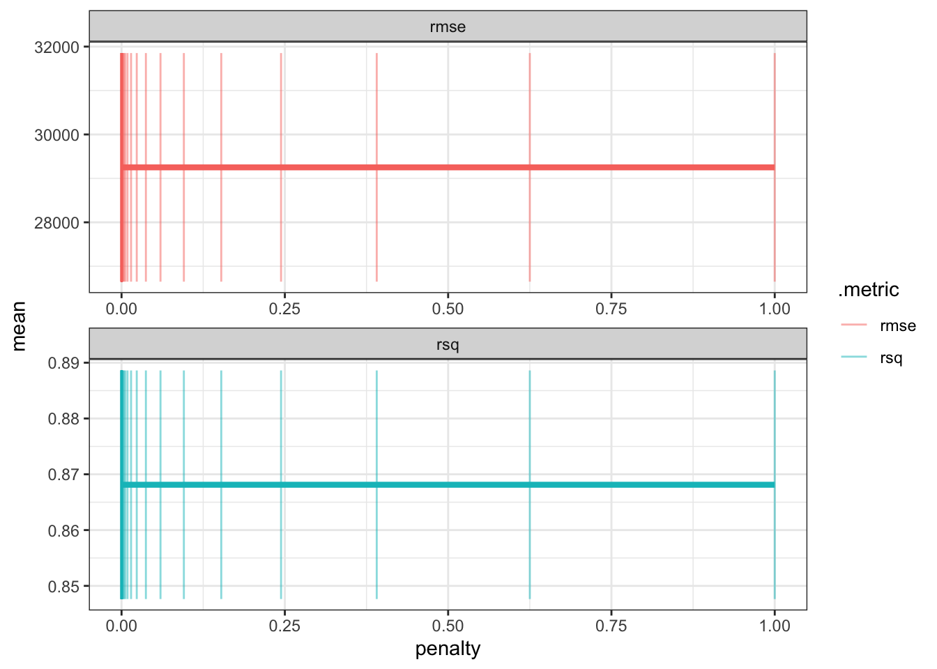
tune_grid()는 하이퍼파라미터 튜닝을 수행하는 함수이다. tune_grid()에는 워크플로우(lasso_wf), 교차검증셋(vb_folds), 튜닝 방식(lambda_grid)이 지정되어야한다. control 옵션은 최종 모델 피팅 후에 pred 값을 저장해주는 옵션이다. 옵션을 지정해놓으면 모델 피팅 후에 ROC plot을 그리거나 다른 기타 그래프로 그리는데 사용할 수 있다.

lasso_res <- tune_grid(
    lasso_wf, 
    resamples = vb_folds, 
    grid = lambda_grid, 
    control = control_grid(save_pred = TRUE), 
)

show_best() 를 이용해서 rmse 기준 best parameter를 볼 수 있다.

show_best(lasso_res, 'rmse')
# A tibble: 5 × 7
   penalty .metric .estimator   mean     n std_err .config              
     <dbl> <chr>   <chr>       <dbl> <int>   <dbl> <chr>                
1 1   e-10 rmse    standard   29251.     5   2602. Preprocessor1_Model01
2 1.60e-10 rmse    standard   29251.     5   2602. Preprocessor1_Model02
3 2.56e-10 rmse    standard   29251.     5   2602. Preprocessor1_Model03
4 4.09e-10 rmse    standard   29251.     5   2602. Preprocessor1_Model04
5 6.55e-10 rmse    standard   29251.     5   2602. Preprocessor1_Model05

penalty parameter에 따라 rmse 값이 어떻게 바뀌는지 ggplot을 이용해서 그래프를 그릴 수 있다.

lasso_res %>% 
    collect_metrics() %>% 
    ggplot(aes(penalty, mean, color = .metric)) + # .metric : rmse 
    geom_errorbar(aes(ymin = mean - std_err, ymax = mean + std_err), alpha = 0.5) + 
    geom_line(size = 1.5, show.legend = F) + 
    facet_wrap(~.metric, scales = 'free', nrow = 2)

튜닝이 끝난 best parameter를 finalize_workflow() 를 이용해서 workflow에 업데이트한다.

best_param <- select_best(lasso_res, 'rmse')
final_lasso <- finalize_workflow(lasso_wf, best_param)
final_lasso
══ Workflow ════════════════════════════════════════════════════════════════════
Preprocessor: Formula
Model: linear_reg()

── Preprocessor ────────────────────────────────────────────────────────────────
sale_price ~ .

── Model ───────────────────────────────────────────────────────────────────────
Linear Regression Model Specification (regression)

Main Arguments:
  penalty = 1e-10
  mixture = 1

Computational engine: glmnet 

최종 모형을 train set에 적합시킨다.

lasso_fit <- fit(final_lasso, data = ames_train_prepped)

마지막으로 test set에 모형을 적합시켜서 결과를 확인한다.

pred_lasso <- 
    predict(lasso_fit, ames_test_prepped) %>% 
    mutate(modelo = "LASSO")

pred_lasso %>% head()
# A tibble: 6 × 2
    .pred modelo
    <dbl> <chr> 
1 208329. LASSO 
2 188538. LASSO 
3  89542. LASSO 
4 213798. LASSO 
5 137118. LASSO 
6 126011. LASSO 

참고 문헌

tidymodel with R bookdown

tidymodel recipe object

How are categorical predictors handled in recipes?

Citation

BibTeX citation:
@online{don2021,
  author = {Don, Don and Don, Don},
  title = {Tidymodels Tutorial},
  date = {2021-03-06},
  url = {https://dondonkim.netlify.app/posts/2021-06-12-tidymodels-tutorial/tidymodels_tutorial.html},
  langid = {en}
}
For attribution, please cite this work as:
Don, Don, and Don Don. 2021. “Tidymodels Tutorial.” March 6, 2021. https://dondonkim.netlify.app/posts/2021-06-12-tidymodels-tutorial/tidymodels_tutorial.html.