library(data.table)
library(sp)
#library(rgeos)
#library(rgdal)
library(tidyverse)
library(tmap)
tmap 패키지 튜토리얼
서울시 따릉이 데이터 불러오기
tutorial을 위해서 서울시 따릉이 데이터를 활용한다.
서울시 따릉이 데이터는 https://data.seoul.go.kr/dataList/OA-13252/F/1/datasetView.do 에서 다운로드가 가능하다.
station <- read_csv('~/Desktop/quarto_blog/posts/data/공공자전거 대여소 정보.csv', locale = locale(encoding = 'CP949'))New names:
Rows: 2082 Columns: 10
── Column specification
──────────────────────────────────────────────────────── Delimiter: "," chr
(4): 월계미륭아파트 정문, 노원구, 노원구 월계동 14, QR dbl (5): 1695,
37.623417, 127.066933, ...8, 10 date (1): 2020-06-17
ℹ Use `spec()` to retrieve the full column specification for this data. ℹ
Specify the column types or set `show_col_types = FALSE` to quiet this message.
• `` -> `...8`colnames(station) <- c('대여소번호', '대여소명', '자치구', '상세주소', 'lat', 'long', '설치시기', 'LCD거치대수', 'QR거치대수', '운영방식')
station %>% head()# A tibble: 6 × 10
대여소번호 대여소명 자치구 상세주소 lat long 설치시기 LCD거치대수
<dbl> <chr> <chr> <chr> <dbl> <dbl> <date> <dbl>
1 2301 현대고등학교 건… 강남구 서울특… 37.5 127. 2017-06-13 10
2 2302 교보타워 버스정… 강남구 서울특… 37.5 127. 2017-06-13 10
3 2303 논현역 7번출구 강남구 서울특… 37.5 127. 2017-06-13 15
4 2304 신영 ROYAL PALA… 강남구 서울특… 37.5 127. 2017-06-13 10
5 2305 MCM 본사 직영점… 강남구 서울특… 37.5 127. 2017-06-13 10
6 2306 압구정역 2번 출… 강남구 서울특… 37.5 127. 2017-06-13 30
# ℹ 2 more variables: QR거치대수 <dbl>, 운영방식 <chr>따릉이 종류에 따라 LCD, QR 방식이 있다. tutorial에서는 LCD 방식의 따릉이 데이터만 이용한다.
station_lcd <- station %>% filter(운영방식 == 'LCD') %>% select(대여소번호, 자치구, LCD거치대수, lat, long)
station_QR <- station %>% filter(운영방식 == 'QR') %>% select(대여소번호, 자치구, QR거치대수, lat, long)
station_lcd %>% dim()
[1] 1531 5서울시군구 SHP 파일 불러오기
shp 파일을 불러올 수 있는 패키지는 여러가지가 있다. 여기서는 rgdal 패키지에 있는 readOGR 함수를 이용한다.
readOGR 함수를 이용해서 데이터를 불러올 때 컴퓨터 셋팅에 따라서 한글이 깨질 수 있다. 한글이 깨질 경우 encoding을 utf-8 로 변경해주면 대부분 해결된다.
areas <- sf::st_read('~/Desktop/quarto_blog/posts/data/서울시군구/TL_SCCO_SIG_W.shp')Reading layer `TL_SCCO_SIG_W' from data source
`/Users/sangdon/Desktop/quarto_blog/posts/data/서울시군구/TL_SCCO_SIG_W.shp'
using driver `ESRI Shapefile'
Simple feature collection with 25 features and 6 fields
Geometry type: POLYGON
Dimension: XY
Bounding box: xmin: 126.7645 ymin: 37.42831 xmax: 127.1838 ymax: 37.7013
Geodetic CRS: WGS 84plot(areas)
shp 파일을 불러오고나서 가장 먼저 확인해야될 것은 crs, 즉 좌표계이다.
좌표계는 구 모양의 지구를 평면인 지도에 투영하는 방법을 지칭한다. 준거타원체의 종류, 타원체의 위치 기준(datum), 투영 방법에 따라 다양한 좌표계가 존재하며, 국가별로 이용하는 좌표계가 따로 존재한다. 따라서 데이터를 병합할 때 좌표계가 다르면 같은 위치여도 부정확한 위치에 좌표가 투영되게 된다.
좌표계를 표시하는 방법은 EPSG 숫자코드 방식과 PROJ4 정형 문자열 방식이 있다. R에서는 좌표계를 지정하는 함수에 따라서 EPSG 숫자코드 방식을 사용할 수도 있고, PROJ4 정형 문자열 방식을 사용할 수 있으므로, 함수에 맞는 방식을 사용해야 한다.
예제를 보면 areas 데이터의 crs는 PROJ4 정형 문자열 방식으로 표시된 +proj=longlat +datum=WGS84 +no_defs이므로 stn.point 데이터의 crs를 해당 좌표계에 대응되는 +init=EPSG:4326로 지정해주었다 (SpatialPointsDataFrame()에 내장되어 있는 CRS()에는 EPSG 숫자코드 방식으로 좌표를 지정해주어야 한다).
EPSG 숫자코드 방식에 대응되는 PROJ4 정형 문자열은 하단 링크를 통해 확인할 수 있다.
SpatialPointsDataFrame()은 기존에 위경도가 내장되어있는 데이터프레임을 SpatialPointDataFrame 형태로 바꾸는 함수이다. 우리가 사용할건 대여소의 위치, 즉 point이므로 위와 같은 데이터의 형태로 바꿔준다. 경우에 따라서SpatialPolygonsDataFrame를 이용할 수도 있다. SpatialPointsDataFrame()에 기존 데이터 프레임의 위경도 정보를 넣어주어야 하는데 주의할 점은 station_lcd[,c(5,4)]처럼 경도, 위도 순으로 넣어주어야 한다.
stn.points <- SpatialPointsDataFrame(station_lcd[,c(5,4)], station_lcd, proj4string = CRS("+init=EPSG:4326"))areas와 stn.point의 위경도를 보면 거의 숫자가 비슷하므로 알맞게 좌표계가 변경되었음을 확인할 수 있다.
tmap 패키지를 이용한 시각화
tmap 패키지는 sp, leaflet 패키지와 잘 연동된다. 시각화는 ggplot의 로직과 거의 비슷하다.
tm_shape : 지도를 불러오는 함수. ggplot()과 비슷함
tm_borders : 지도 테두리를 그리는 함수
- alpha = 선의 선명도
tm_dots : 지도에 점을 찍는 함수
style = ‘equal’ : 변수의 range를 n으로 나눔
style = ‘pretty’ : 변수의 range를 균등한 값으로 나눔
style = ‘quantile’ : 각 그룹에 동일한 case 개수 할당
style = ‘jenks’ : 데이터에서 nature breaks 를 찾음
style = ‘Cat’ : 변수가 범주형 변수일 경우
n = 5(default) : interval 수 지정
palette = 점 색 조절
scale = 점 크기 조절
tm_compass : 방향 표시
tm_layout : legend 커스텀하는 함수
legend.text.size = legend 글씨 크기 조절
legend.title.size = legend 제목 크기 조절
frame = legend에 테두리 넣을 건지 유무
tmap_options(check.and.fix = TRUE)
tm_shape(areas) +
  tm_borders(alpha = 1) +
  tm_shape(stn.points) + tm_dots(col = 'LCD거치대수', palette = 'Reds', style = 'quantile', scale = 2.5) +
  tm_compass()+
  tm_layout(legend.text.size = 0.8, legend.title.size = 1.1, frame = FALSE)
Warning: The shape areas is invalid. See sf::st_is_valid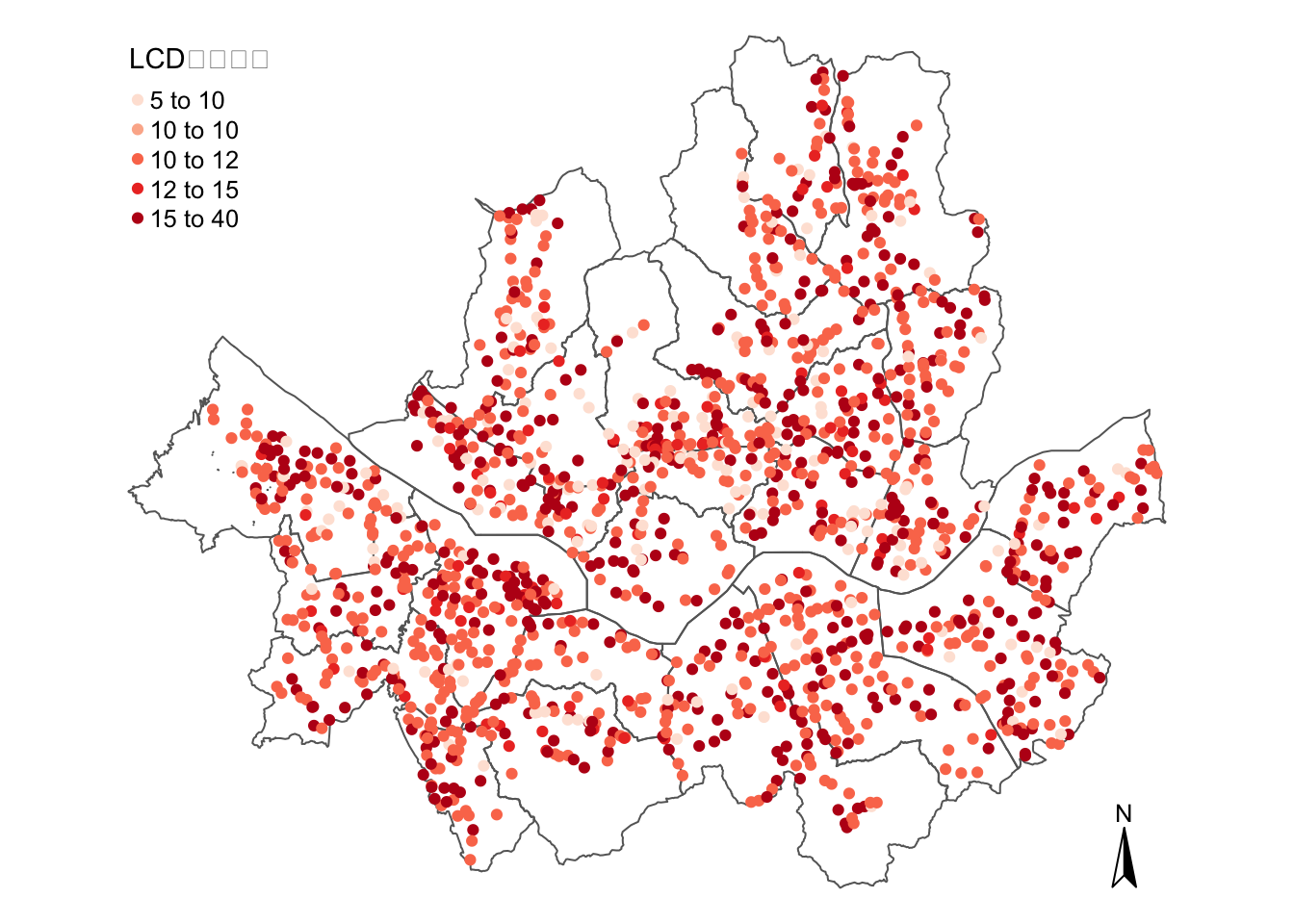
leaflet 패키지를 이용한 interactive plot
tmap은 leaflet 패키지와 간단하게 연동이 가능하다. tmap_mode를 지정하고 tmap 함수를 그대로 적용하면 된다.
library(leaflet)
tmap_mode("view")
tmap mode set to interactive viewingtm_shape(areas) +
tm_borders(alpha = 0.5) +
tm_shape(stn.points) + tm_dots(col = 'LCD거치대수', palette = 'Reds', style = 'quantile', scale = 2.5) +
tm_compass()+
tm_layout(legend.text.size = 0.8, legend.title.size = 1.1, frame = FALSE)Compass not supported in view mode.Warning: The shape areas is invalid. See sf::st_is_valid좌표계 개념 참고 : https://www.biz-gis.com/index.php?mid=pds&document_srl=65754
대응되는 좌표계 참고 : https://statkclee.github.io/spatial/geo-spatial-r.html
다양한 좌표계 관련 참고 : https://www.osgeo.kr/17
Citation
BibTeX citation:
@online{don2024,
  author = {Don, Don and Don, Don},
  title = {Tmap in {R}},
  date = {2024-03-09},
  url = {https://dondonkim.netlify.app/posts/2021-06-12-tmap-in-r/tmap.html},
  langid = {en}
}
For attribution, please cite this work as:
Don, Don, and Don Don. 2024. “Tmap in R.” March 9, 2024. https://dondonkim.netlify.app/posts/2021-06-12-tmap-in-r/tmap.html.