library(tidyverse)
library(easystats)
library(GGally)
library(skimr)
library(broom)
library(ggdag)
library(dagitty)
library(broom)

#data("msleep")
partial \(R^2\)
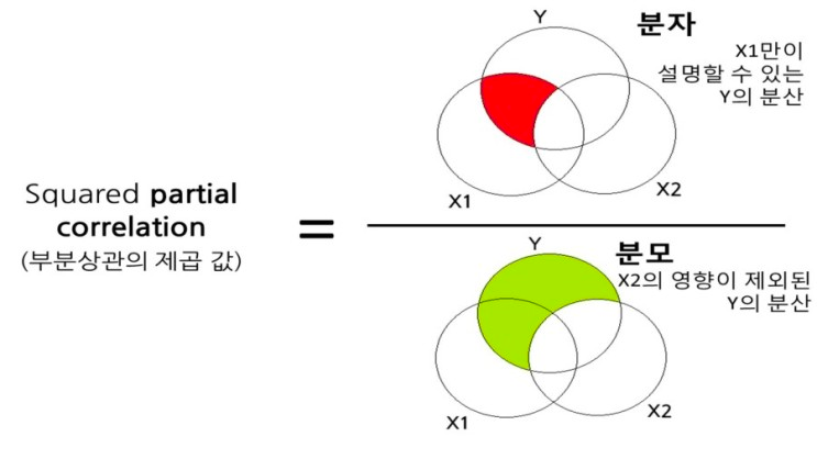
먼저 \(R^2\)는 \(Y\)의 총 분산 중 \(X\)에 의해 설명되는 분산의 비율을 의미합니다(오른쪽 그림 참고).
partial \(R^2\)는 “partial”의 의미 그대로 다른 변수들의 관계를 제거하고 \(Y\) 의 변동에 기여하는 순수한 \(X\)의 변동을 의미합니다. partial \(R^2\)는 sensitivity analysis에 이용할 수 있습니다.
set.seed(1)
dagify(Y ~ X1,
       X1 ~ eX1,
       eX1 ~~ eY,
       Y ~ eY,
       Y ~ X2,
       X1 ~ X2) %>%
  ggdag() +
    theme_minimal()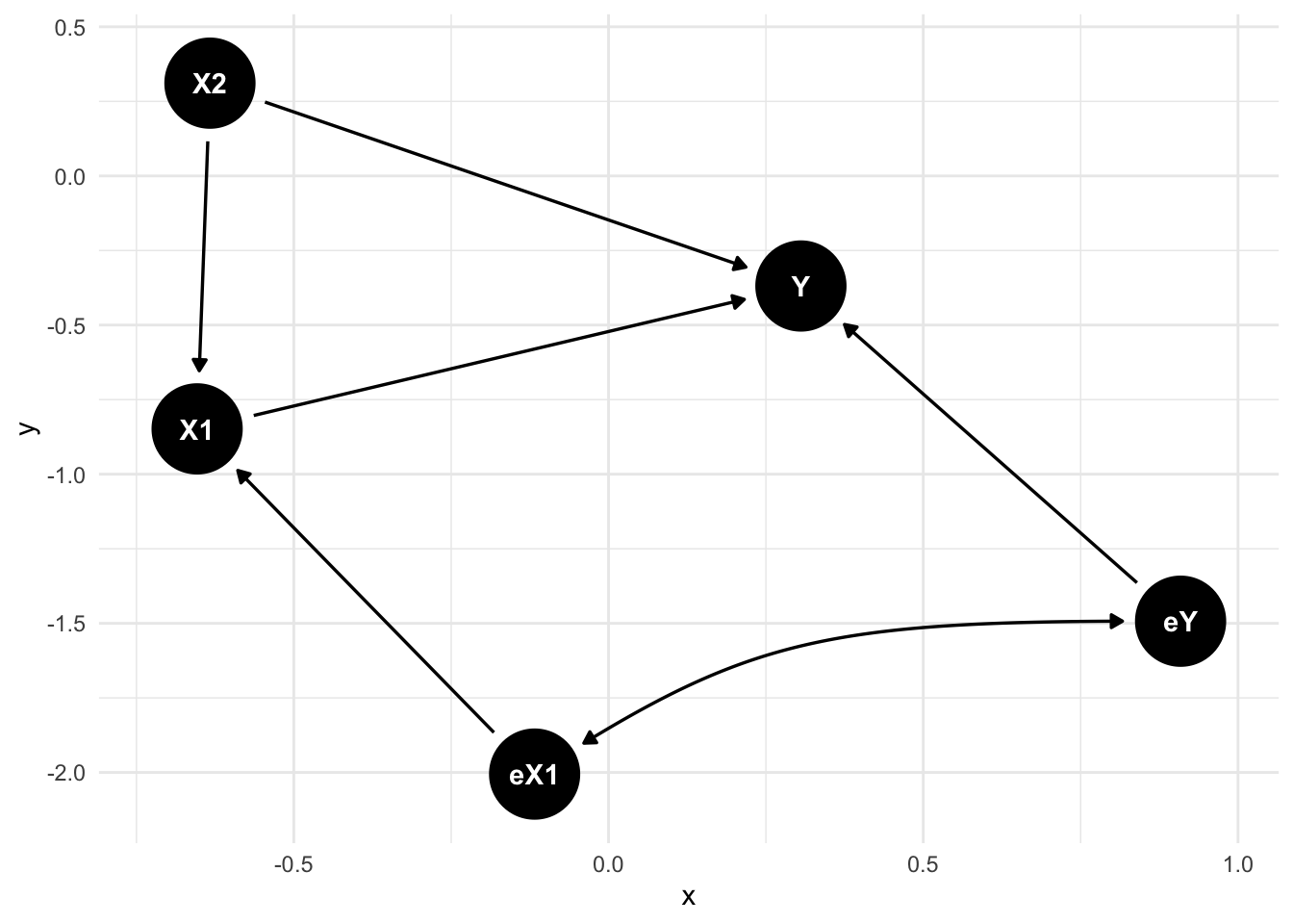
그림을 통해 보면 X2는 confounder로 X1과 Y에 동시에 영향을 주는 변수입니다. 이 때, confounder의 효과를 제거하고 Y ~ X1의 효과를 보려고 합니다. 이 경우 partial \(R^2\)를 이용할 수 있습니다.
partial \(R^2\)는 Y의 변동 중 confounder X2을 통제했을 때, X1가 설명하는 변동의 비율을 의미합니다.
\[ R^2_{Y \sim X_1|X_2} = \frac{SSE(X_2) - SSE(X_1, X_2)}{SSE(X_2)} \]
Example
data description
포유류의 수면과 관련된 데이터
sleep_total : 총 수면 시간 (\(Y\))
brainwt : 뇌의 무게
bodywt : 체중
brainwt(\(X_1\))의 partial \(R^2\)를 계산해보겠습니다.
dat <- read_csv("./msleep.csv")corr <- dat %>%
cor()
corr sleep_total brainwt bodywt
sleep_total 1.0000000 -0.6806058 -0.6810127
brainwt -0.6806058 1.0000000 0.9448724
bodywt -0.6810127 0.9448724 1.0000000먼저 correlation(zero-order-correlation)를 보면 sleep_total과 brainwt의 correlation는 \(-0.68\)로 강한 음의 상관관계가 존재하는 것을 볼 수 있습니다. correlation 패키지에 partial correlation을 계산하는 함수가 이미 있으므로 이용해보겠습니다.
cor_to_pcor(corr) sleep_total brainwt bodywt
sleep_total 1.0000000 -0.1548778 -0.1580967
brainwt -0.1548778 1.0000000 0.8972459
bodywt -0.1580967 0.8972459 1.0000000sleep_total과 brainwt의 partial correlation는 \(-0.15\)로 이전 zero-order-correlation과 달리 약한 음의 상관관계가 존재하는 것을 볼 수 있습니다.
cor_to_pcor(corr)^2 sleep_total brainwt bodywt
sleep_total 1.00000000 0.02398713 0.02499458
brainwt 0.02398713 1.00000000 0.80505014
bodywt 0.02499458 0.80505014 1.00000000partial \(R^2\)를 구해보면 \(0.023\) 정도인 것을 볼 수 있습니다. 변수의 의미를 보면 brainwt(\(X_1\))는 bodywt(\(X_2\))의 일부입니다. 따라서 bodywt(\(X_2\))를 통제했을 때, brainwt(\(X_1\))가 설명하는 \(Y\)의 변동은 미미하다고 볼 수 있습니다.
ANOVA table을 이용해서 다시 계산해보겠습니다.
fit_f <- lm(sleep_total ~ ., dat)
fit_b <- lm(sleep_total ~ bodywt, dat)
fit_f_anov <- anova(fit_f) %>% tidy()
fit_b_anov <- anova(fit_b) %>% tidy()

(fit_b_anov$sumsq[2] - fit_f_anov$sumsq[3])/fit_b_anov$sumsq[2]
[1] 0.02398713결과는 동일한 것을 확인할 수 있습니다.
fit1 <- lm(sleep_total ~ bodywt, dat)
fit2 <- lm(brainwt ~ bodywt, dat)

r1 <- augment(fit1)$.resid
r2 <- augment(fit2)$.resid

cor(r1, r2)^2
[1] 0.02398713semi partial(or part) \(R^2\)
set.seed(12)
dagify(X1 ~ X2,
       X1 ~ eX1,
       Y ~ X1,
       Y ~ eX1) %>%
  ggdag() +
    theme_minimal()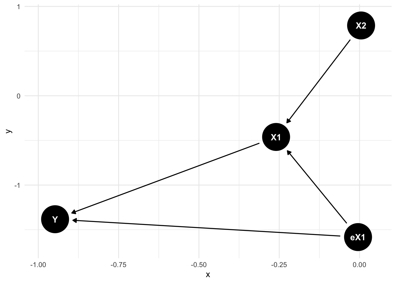
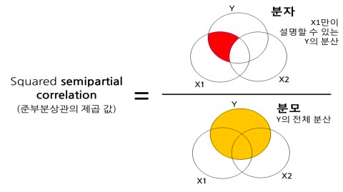
semi partial(or part) \(R^2\)는 Y의 변동 중 변수를 추가했을 때, 추가한 변수가 설명하는 변동의 비율을 의미합이다. semi partial(or part) \(R^2\)와 partial \(R^2\)의 차이는 confounder가 Y와 \(\mathbf{X}\)에 동시에 영향을 미치는지, 혹은 \(\mathbf{X}\)에만 영향을 미치는지로 볼 수 있습니다.
\[ sr_1^2 = r_{y, (1.2)}^2 = (\frac{r_{y.1} - r_{y.2} \cdot r_{1.2}}{\sqrt{1 - r^2_{1.2}}})^2 \]
\[ sr_1^2 = R^2_{y, 1.2} - r^2_{y.2} \]
Example
sleep_total(\(Y\))의 분산 중 brainwt(\(X_1\))가 설명하는 순수 비율을 계산하려고 합니다. (bodywt(\(X_2\)) 제외)
cor_to_spcor(corr, cov = sapply(dat, sd)) sleep_total brainwt bodywt
sleep_total 1.00000000 -0.1134126 -0.1158295
brainwt -0.05071300 1.0000000 0.6573670
bodywt -0.05176701 0.6570276 1.0000000semi-partial correlation을 구해보면 partial correlation과 비슷하게 \(sr_1^2 = -0.11\)로 correlation과 큰 차이가 있는 것을 볼 수 있습니다.
cor_to_spcor(corr, cov = sapply(dat, sd))^2 sleep_total brainwt bodywt
sleep_total 1.000000000 0.01286242 0.01341648
brainwt 0.002571808 1.00000000 0.43213138
bodywt 0.002679823 0.43168533 1.00000000semi-partial \(R^2\)를 구해보면 \(0.012\)입니다. 이전과 마찬가지로 변수의 의미를 보면 brainwt(\(X_1\))는 bodywt(\(X_2\))값의 일부입니다. 따라서 brainwt(\(X_1\))가 설명하는 \(Y\)의 변동은 미미하다고 볼 수 있습니다.
fit1 <- lm(sleep_total ~ bodywt + brainwt, dat)
fit2 <- lm(sleep_total ~ bodywt, dat)

r2_y12 <- broom::glance(fit1)$r.squared
r2_y2 <- broom::glance(fit2)$r.squared

r2_y12 - r2_y2
[1] 0.01286242이는 단순하게 full model의 \(R^2\)에서 \(Y \sim X_1\)의 \(R^2\)의 차이를 통해서도 구할 수 있다(\(R^2_{y, 1.2} - r^2_{y.2} = 0.4766408 - r2_y2\))
fit3 <- lm(brainwt ~ bodywt, dat)

cor(augment(fit3)$.resid, dat$sleep_total)^2
[1] 0.01286242또는 \(X_1 \sim X_2\)의 잔차(\(X_1\)에서 \(X_2\)가 설명하는 부분을 제외한 부분)와 \(Y\)와의 상관계수의 제곱을 통해서도 마찬가지로 구할 수 있다.
참고자료
https://brendanhcullen.github.io/psy612/lectures/7-partial.html#25
https://rpubs.com/KwonPublishing/249631
https://easystats.github.io/correlation/reference/cor_to_pcor.html
https://m.blog.naver.com/PostView.naver?isHttpsRedirect=true&blogId=soowon0109&logNo=30173631827
Citation
BibTeX citation:
@online{don2022,
  author = {Don, Don and Don, Don},
  title = {Partial {R} Squared},
  date = {2022-08-31},
  url = {https://dondonkim.netlify.app/posts/2022-08-31-partial-correlation/partial_corr.html},
  langid = {en}
}
For attribution, please cite this work as:
Don, Don, and Don Don. 2022. “Partial R Squared.” August
31, 2022. https://dondonkim.netlify.app/posts/2022-08-31-partial-correlation/partial_corr.html.