library(tidyverse)Randomly Over Sampling Examples(ROSE)
ROSE는 smooth boostrap을 적용하여 리샘플링하는 방법입니다. smooth boostrap이란 resampling된 관측치에 평균이 0이고 정규분포를 따르는 아주 작은 양의 random noise을 더해 새로운 표본을 생성하는 원리를 따릅니다. ROSE는 oversampling과 undersampling 기법을 결합하여 소수 클래스는 늘리고, 다수클래스는 줄인 새로운 샘플을 생성합니다. 어떻게 계산되는지 알아보겠습니다.
먼저 iris 데이터를 불러오겠습니다.
2차원 시각화를 위해서 Sepal.Length, Sepal.Width, Species 변수만 이용하겠습니다.
iris$Species %>% unique()[1] setosa versicolor virginica
Levels: setosa versicolor virginicaX <- iris[, c(1, 2, 5)] %>%
filter(Species %in% c("setosa", "versicolor") & row_number() %in% c(1:20, 51:100)) %>%
mutate(Species = factor(Species, labels = c("No", "Yes")))X %>%
ggplot(aes(x = Sepal.Length, y = Sepal.Width, color = Species)) +
geom_point()
No는 소수 클래스이고, Yes는 다수 클래스입니다. ROSE를 적용하고 결과를 살펴보겠습니다.
ROSE는 rose.real() 함수를 통해서 계산됩니다. 하나씩 어떻게 계산되는지 살펴보겠습니다.
rose.real <- function(X, hmult=1, n, q = NCOL(X), ids.class, ids.generation)
{
    X <- data.matrix(X)
    n.new <- length(ids.generation)
    cons.kernel <- (4/((q+2)*n))^(1/(q+4))

    if(q!=1)
        H <- hmult*cons.kernel*diag(apply(X[ids.class,], 2, sd), q) # 3x3
    else
        H <- hmult*cons.kernel*sd(X[ids.class,])

    Xnew.num <- matrix(rnorm(n.new*q), n.new, q)%*%H
    Xnew.num <- data.matrix(Xnew.num + X[ids.generation,])
    Xnew.num
}
rose.real(X, hmult=1, n, q, ids.class, ids.generation)
X : numeric matrix
hmult : smoothing parameter
n : 소수 클래스의 수
q : 수치형 칼럼의 수
ids.class : 소수 클래스의 index
ids.generation : 복원 추출한 소수클래스의 index
classx <- sapply(as.data.frame(X), class)
classx
Sepal.Length Sepal.Width Species
"numeric" "numeric" "factor" id.num <- which(classx=="numeric" | classx=="integer")
id.numSepal.Length Sepal.Width
1 2 d <- NCOL(X)
hmult = 1
p <- 0.5
N <- nrow(X)
n.mino.new <- sum(rbinom(N, 1, p)) #number of new minority class examples
n.mino.new[1] 37n.majo.new <- N-n.mino.new #number of new minority class examples
n.majo.new[1] 33majoY <- "Yes" # major label
minoY <- "No" # minor label
ind.mino <- which(X$Species == minoY)
ind.majo <- which(X$Species == majoY)
ind.mino [1] 1 2 3 4 5 6 7 8 9 10 11 12 13 14 15 16 17 18 19 20ind.majo [1] 21 22 23 24 25 26 27 28 29 30 31 32 33 34 35 36 37 38 39 40 41 42 43 44 45
[26] 46 47 48 49 50 51 52 53 54 55 56 57 58 59 60 61 62 63 64 65 66 67 68 69 70n <- length(ind.majo)
q <- d-length( which(classx=="factor"))
q[1] 2복원추출을 활용하여, 소수 클래스는 관측치의 수를 늘리고, 다수 클래스는 관측치의 수를 줄입니다.
id.majo.new <- sample(ind.majo, n.majo.new, replace=TRUE)
id.mino.new <- sample(ind.mino, n.mino.new, replace=TRUE)
rose.real() 함수에서 cons.kernel 값은 n(소수 클래스의 수)와 q(수치형 칼럼의 수)) 로 계산됩니다.
n <- length(ind.mino)
q <- d-length( which(classx=="factor"))
cons.kernel <- (4/((q+2)*n))^(1/(q+4))
cons.kernel
# > cons.kernel
# [1] 0.6069622
수치형 변수만 있어야 하므로 X에서 수치형 변수만 filtering 해줍니다. X matrix의 각 칼럼별 표준편차를 구한 후 사전에 지정한 hmult와 cons.kernel과 함께 곱합 matrix H를 생성합니다.
X <- X[,id.num]
X[1:3, ]
#   Sepal.Length Sepal.Width
# 1          5.1         3.5
# 2          4.9         3.0
# 3          4.7         3.2
H <- hmult*cons.kernel*diag(apply(X[ind.mino,], 2, sd), q)
# > H
# [,1] [,2]
# [1,] 0.2592196 0.0000000
# [2,] 0.0000000 0.2472168matrix H는 synthetic sample을 생성할 때, random noise의 크기를 조절하는 역할을 합니다. 따라서 \(Hmult \approx 0\)이면 새로운 표본을 생성할 때, 작은 random noise가 더해지므로, 기존의 관측치의 값과 거의 유사한 표본을 생성하고, \(Hmult \approx 1\)이면 새로운 표본을 생성할 때, 큰 random noise가 더해지므로, 기존의 관측치 주변의 값을 새로운 표본으로 생성합니다.
n.new <- length(id.mino.new)
Xnew.num <- matrix(rnorm(n.new*q), n.new, q)%*%H
# > Xnew.num %>% head()
#             [,1]        [,2]
# [1,]  0.04899544 -0.31797929
# [2,]  0.11534283 -0.04240093
# [3,] -0.05767842 -0.11889093
# [4,] -0.02200680  0.18249786
# [5,]  0.13977148  0.09139938
# [6,]  0.16442458  0.06085837
평균이 0인 정규분포와 H matrix를 곱한 random noise matrix를 생성합니다.
Xnew.num <- data.matrix(Xnew.num + X[id.mino.new,])
# > Xnew.num %>% head()
#     Sepal.Length Sepal.Width
# 5       5.048995    3.282021
# 6       5.515343    3.857599
# 9       4.342322    2.781109
# 1       5.077993    3.682498
# 12      4.939771    3.491399
# 5.1     5.164425    3.660858
# > X %>% head()
# Sepal.Length Sepal.Width
# 1 5.1 3.5
# 2 4.9 3.0
# 3 4.7 3.2
# 4 4.6 3.1
# 5 5.0 3.6
# 6 5.4 3.9random noise를 더한 새롭게 생성한 관측치와 기존의 관측치 값을 대략적으로 비교해보면 관측치 주변 이웃으로 새로운 관측치가 생성되는 것을 볼 수 있습니다.
rose_result <- rose.real(X[,id.num],
                         hmult=1,
                         n=length(ind.mino),
                         q=q,
                         ids.class=ind.mino,
                         ids.generation=id.mino.new)
X %>%
ggplot() +
geom_point(aes(x = Sepal.Length, y = Sepal.Width, color = Species)) +
geom_point(aes(x = Sepal.Length, y = Sepal.Width), data = rose_result %>% as.data.frame())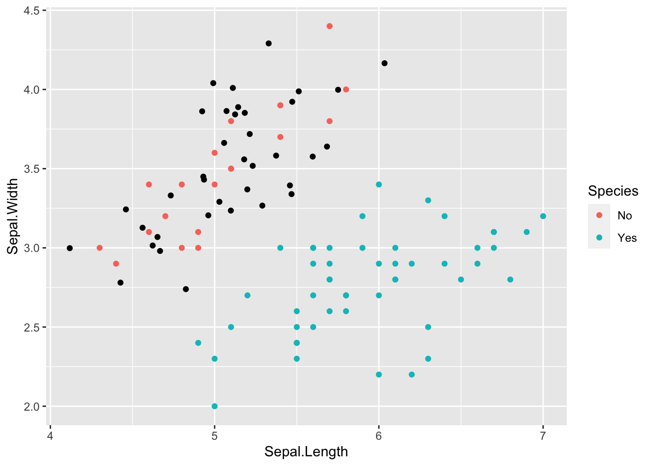
hmult=0.01로 설정하면 기존 관측치와 가까운 새로운 관측치를 생성하는 것을 볼 수 있습니다.
rose_result2 <- rose.real(X[,id.num],
                         hmult=0.01,
                         n=length(ind.mino),
                         q=q,
                         ids.class=ind.mino,
                         ids.generation=id.mino.new)
X %>%
ggplot() +
geom_point(aes(x = Sepal.Length, y = Sepal.Width, color = Species)) +
geom_point(aes(x = Sepal.Length, y = Sepal.Width), data = rose_result2 %>% as.data.frame())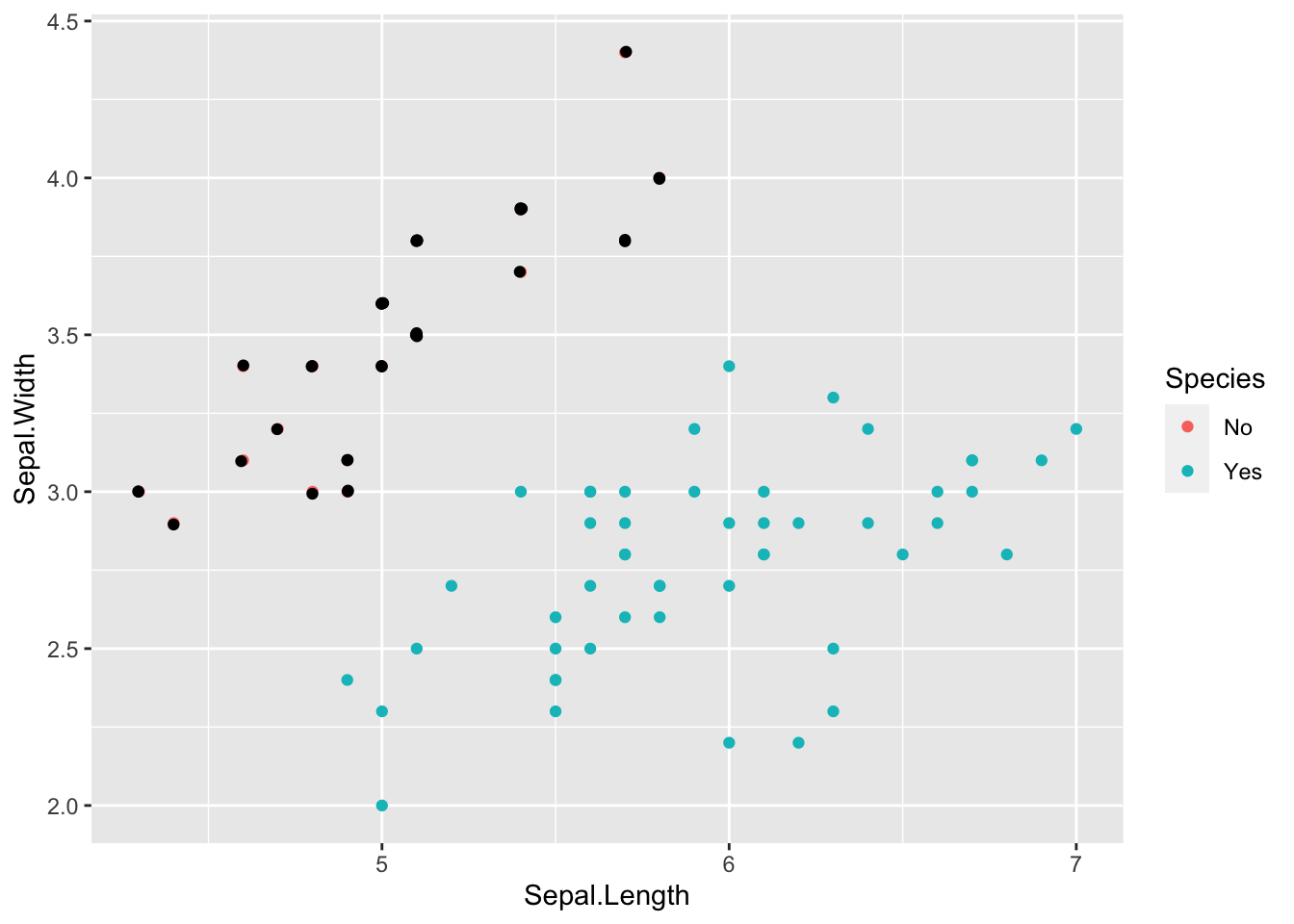
Xnew <- data.frame(X[c(id.majo.new, id.mino.new),])
Xnew %>% dim()
[1] 70 3hmult.majo = 1
hmult.mino = 1소수 클래스와 다수 클래스 각각에 rose.real() 함수를 적용합니다. 소수 클래스는 늘리고, 다수 클래스는 줄여서 Xnew 데이터를 새롭게 생성합니다.
Xnew[1:n.majo.new, id.num] <- rose.real(X[,id.num], hmult=hmult.majo, n=length(ind.majo), q=q, ids.class=ind.majo, ids.generation=id.majo.new)
#Xnew[1:n.majo.new, id.num] %>% dim() : 80, 2
#
Xnew[(n.majo.new+1):N, id.num] <- rose.real(X[,id.num], hmult=hmult.mino, n=length(ind.mino), q=q, ids.class=ind.mino, ids.generation=id.mino.new)
X %>%
ggplot() +
geom_point(aes(x = Sepal.Length, y = Sepal.Width, color = Species)) +
geom_point(aes(x = Sepal.Length, y = Sepal.Width, color = Species), data = Xnew)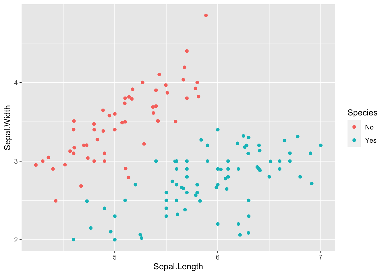
Xnew %>%
    ggplot() +
    geom_point(aes(x = Sepal.Length, y = Sepal.Width, color = Species))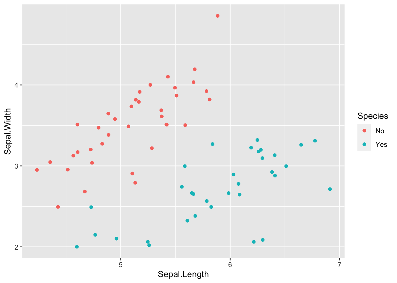
X$Species %>% table().
No Yes
20 50 Xnew$Species %>% table().
No Yes
37 33 ROSE package 이용
result <- ROSE::ROSE(Species~., data = X)
result$data %>%
    ggplot() +
    geom_point(aes(x = Sepal.Length, y = Sepal.Width, color = Species))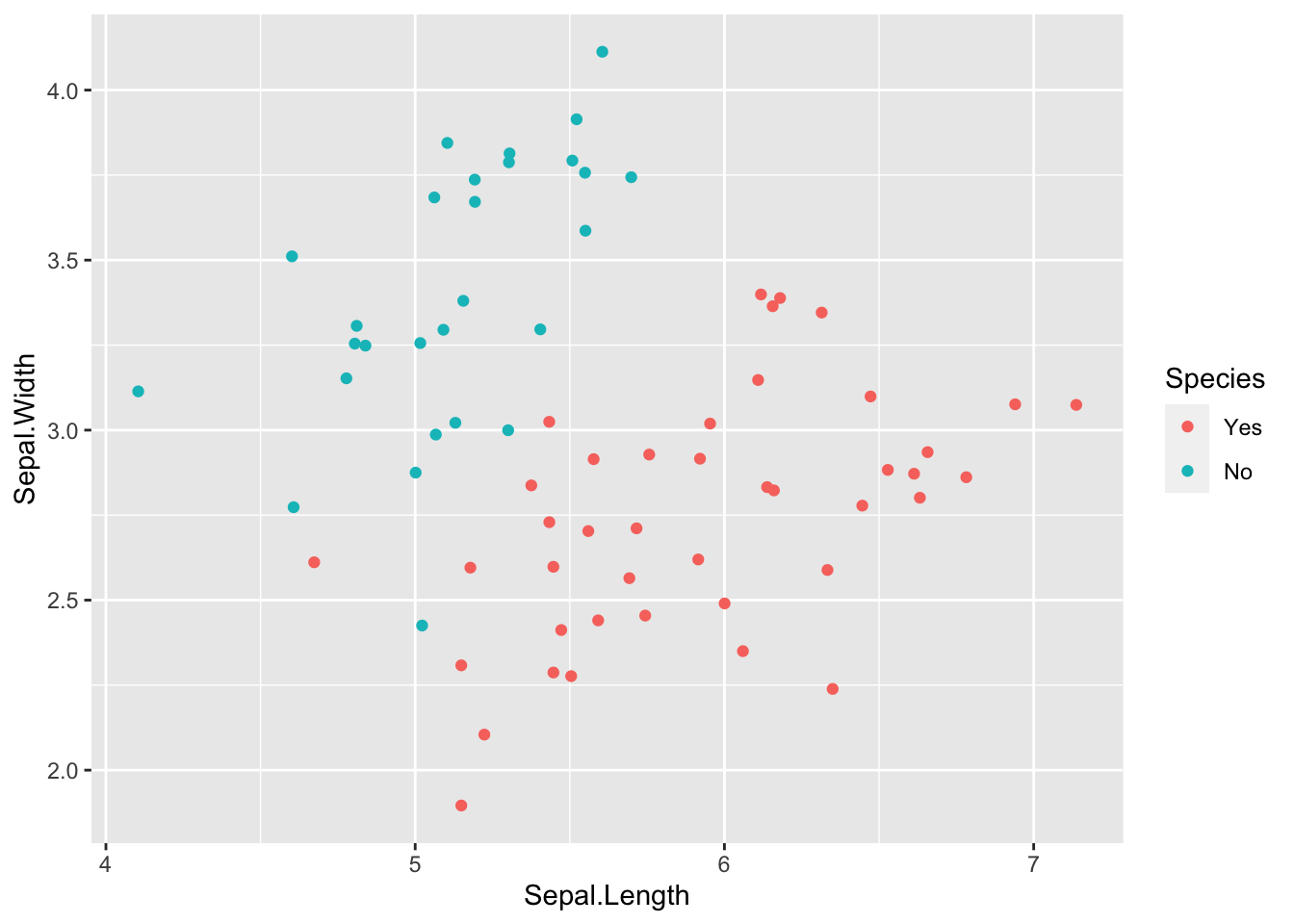
result$data$Species %>% table().
Yes No
42 28 X$Species %>% table().
No Yes
20 50 참고 자료
https://github.com/cran/ROSE/blob/master/R/data_balancing_funcs.R
Citation
BibTeX citation:
@online{don2022,
  author = {Don, Don and Don, Don},
  title = {ROSE},
  date = {2022-11-16},
  url = {https://dondonkim.netlify.app/posts/2022-11-16-ROSE/rose.html},
  langid = {en}
}
For attribution, please cite this work as:
Don, Don, and Don Don. 2022. “ROSE.” November 16, 2022. https://dondonkim.netlify.app/posts/2022-11-16-ROSE/rose.html.