Sensitive Analysis

일반적으로 관찰 데이터로 인과추론 분석을 할 때에는 관측되지 않은 교란 요인이 없다는 가정 하에서 분석을 진행합니다. 일반적으로 이러한 가정은 만족될 수 없습니다. 따라서 가정이 위반되었을 때, 인과 관계에 미치는 영향을 정량적으로 확인하는 절차, 즉 강건성을 확인하는 절차가 필요합니다.

이것을 측정하기 위해 다음과 같은 질문을 해볼 수 있습니다.

관찰 데이터로 추정한 인과효과를 $0$ 으로 만들기 위해서 관찰되지 않은 교란요인이 $T$ 와 $Y$ 에 얼마나 많은 영향을 끼쳐야 하는가?

민감도분석은 이러한 질문에 답을 하기 위한 정량적인 분석을 수행하는 것입니다.

Sensitivity Basiscs in Linear Setting

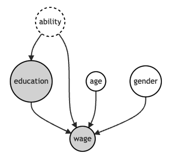
먼저 가장 간단한 세팅으로 linear setting을 고려해보겠습니다. 오른쪽 그림을 보면 $W$ 는 관찰된 교란요인이고, $U$ 는 관찰되지 않은 교란요인을 나타냅니다. $U$ 의 효과를 무시했을 때, 나타나는 편향은 어느 정도일까요?

linear setting에서 $T$ 와 $Y$ 는 다음과 같이 표현할 수 있습니다.

$\begin{aligned} T := α_{w} W + α_{u} U \\ Y := β_{w} W + β_{u} U + δ T \end{aligned}$

먼저 $T, U$ 가 주어졌을 때를 가정하면, ATE는 $δ$ 로 계산됩니다.

$E [Y (1) - Y (0)] = E_{W, U} [E [Y | T = 1, W, U] - E [Y | T = 0, W, U]] = δ$

하지만 $U$ 는 관찰할 수 없는 교란요인이므로, 실제로는 $W$ 만 조정할 수 있습니다. 따라서 $U$ 의 영향으로 confounding bias가 $\frac{β_{u}}{α_{u}}$ 만큼 발생합니다.

$E_{W} [E [Y | T = 1, W] - E [Y | T = 0, W]] - E_{W, U} [E [Y | T = 1, W, U] - E [Y | T = 0, W, U]] = \frac{β_{u}}{α_{u}}$

$p r o o f$

$\begin{aligned} E_{W} [E [Y | T = t, W]] & = E_{W} [E [β_{w} W + β_{u} U + δ T | T = t, W]] \\ = E_{W} [β_{w} W + β_{u} E [U | T = t, W] + δ t] \\ = E_{w} [β_{w} W + β_{u} \frac{t - α_{w} W}{α_{u}} + δ t] \\ = E_{w} [β_{w} W + \frac{β_{u}}{α_{u}} t - \frac{β_{u} α_{w}}{α_{u}} W + δ t] \\ = β_{w} E [W] + \frac{β_{u}}{α_{u}} t - \frac{β_{u} α_{w}}{α_{u}} E [W] + δ t \\ = (δ + \frac{β_{u}}{α_{u}}) t + (β_{w} - \frac{β_{u} α_{w}}{α_{u}}) E [W] \end{aligned}$

$\begin{aligned} E_{W} [E [Y | T = 1, W] - E [Y | T = 0, W]] \\ = (δ + \frac{β_{u}}{α_{u}}) (1) + (β_{w} - \frac{β_{u} α_{w}}{α_{u}}) E [W] - [(δ + \frac{β_{u}}{α_{u}}) (0) + (β_{w} - \frac{β_{u} α_{w}}{α_{u}}) E [W]] \\ = δ + \frac{β_{u}}{α_{u}} \end{aligned}$

$\begin{aligned} B i a s & = E_{W} [E [Y | T = 1, W] - E [Y | T = 0, W]] \\ - E_{W, U} [E [Y | T = 1, W, U] - E [Y | T = 0, W, U]] \\ = δ + \frac{β_{u}}{α_{u}} - δ \\ = \frac{β_{u}}{α_{u}} \end{aligned}$

Sensitivity Contour Plots

true ATE인 $δ$ 는 아래와 같이 다시 정리할 수 있습니다.

$E_{W} [E [Y | T = 1, W] - E [Y | T = 0, W]] = δ + \frac{β_{u}}{α_{u}}$

$\begin{array}{r} δ = E_{W} [E [Y | T = 1, W] - E [Y | T = 0, W]] - \frac{β_{u}}{α_{u}} \end{array}$ 식을 한번 더 해석해보면 다음과 같습니다.

$U$ 에 의해 생기는 bias인 $\frac{β_{u}}{α_{u}}$ 이 크다면 $E_{W} [E [Y | T = 1, W] - E [Y | T = 0, W]]$ 는 상쇄되고, $δ$ 는 $0$ 에 가까워짐
$U$ 에 의해 생기는 bias인 $\frac{β_{u}}{α_{u}}$ 이 작다면 $E_{W} [E [Y | T = 1, W] - E [Y | T = 0, W]]$ 는 크게 변화하지 않고, $δ$ 는 $E_{W} [E [Y | T = 1, W] - E [Y | T = 0, W]]$ 과 큰 차이가 없음

이에 대해서 그래프로 나타내보면 다음과 같습니다.

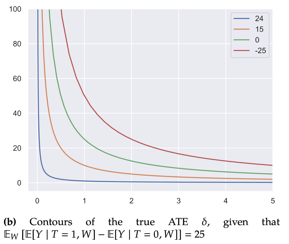
그림은 ( $\frac{1}{α_{u}}$ , $β_{u}$ )에 따른 $δ$ 의 변화 그래프입니다. 먼저 green curve 값을 해석해보겠습니다. $E_{W} [E [Y | T = 1, W] - E [Y | T = 0, W]] = 25$ 로 고정했을 때, $\frac{1}{α_{u}} = 1$ 이고, $β_{u} = 25$ 라면 $δ = 0$ 이 됩니다.

따라서 green curve일 경우 ( $\frac{1}{α_{u}}$ , $β_{u}$ )의 변화에 따른 $δ = 0$ 일 때에 해당하는 곡선입니다. $δ = 0$ 이라는 의미는 관찰되지 않은 교란 요인 $U$ 에 의해 $E_{W} [E [Y | T = 1, W] - E [Y | T = 0, W]]$ 을 전부 설명한다는 의미와 같으며, $U$ 는 강력한 교란요인이라고 볼 수 있습니다.

결론적으로 green curve에 가까워지거나 혹은 green curve를 넘어설 경우 교란요인에 의해 영향을 많이 받으므로, 강건성이 떨어진다고 볼 수 있습니다.

정리하면, 관찰되지 않은 교란요인이 treatment와 outcome에 대해 미치는 영향의 방향은 알 수 없습니다. 이에 따라 민감도 분석에서는 관찰되지 않은 교란요인의 크기를 고려합니다. 위의 그림 예시처럼 민감도 분석을 통해 추정된 효과를 없앨 정도로 추정량을 변경하려면 관찰되지 않은 교란요인의 크기가 어느 정도여야 하는지를 확인할 수 있고, 도메인 지식을 활용하여 추정된 효과의 강건성을 주관적으로 결정할 수 있습니다.

Sensemakr

paper에서는 partial $R^{2}$ 를 활용해서 linear regression에서 민감도분석을 수행하고 리포팅하기 위한 새로운 방식을 제안합니다.

주요 기여사항

Robustness value 개발
partial $R^{2}$ 를 활용한 민감도분석 툴 개발
extreme scenario에 대한 분석 그래프 개발

해당 논문 저자가 개발한 툴은 R, Python, Stata 등에서 이용할 수 있습니다.

python : dowhy, PySensemakr
R : sensemakr

Example

참고 : https://matteocourthoud.github.io/post/ovb/
교육기간과 임금 사이의 관계에 관심이 있음
교육기간과 임금 사이에는 많은 unobserved confounder가 존재함
예시를 위해 unobserved confounder로 ability가 있다고 가정
ability는 omitted variable이지만 education과 wage에 영향을 미친다는 것을 알고 있다고 가정함

library(sensemakr)
library(tidyverse)

#setwd("./posts/2023-02-07-sensitivity-analysis")
df <- read.csv("ex_data.csv")[, -1] %>% 
    mutate(gender = as.factor(gender))
df %>% head(2)

  age gender education wage
1  62   male         6 3800
2  44   male         8 4500

fit <- lm(wage ~ ., df)
summary(fit)


Call:
lm(formula = wage ~ ., data = df)

Residuals:
    Min      1Q  Median      3Q     Max 
-958.27 -194.90   -1.32  256.00  967.54 

Coefficients:
            Estimate Std. Error t value Pr(>|t|)    
(Intercept)  2657.89     445.00   5.973 3.18e-07 ***
age            12.31       6.11   2.015   0.0498 *  
gendermale    335.11     132.69   2.526   0.0151 *  
education      95.94      38.75   2.476   0.0170 *  
---
Signif. codes:  0 '***' 0.001 '**' 0.01 '*' 0.05 '.' 0.1 ' ' 1

Residual standard error: 455.1 on 46 degrees of freedom
Multiple R-squared:  0.2549,    Adjusted R-squared:  0.2063 
F-statistic: 5.246 on 3 and 46 DF,  p-value: 0.003379

회귀분석 결과, 추정된 ATE는 약 $96$ 으로, 교육 기간이 한 단위 증가할 때, 임금은 약 96 증가합니다(education = $95.94$ ). 하지만 실제로는 관찰되지 않은 교란요인(ability)이 존재하므로, 해당 추정량은 편향 추정량입니다(해당 데이터는 가상의 데이터이므로, 실제로는 수 많은 교란요인이 존재합니다).

관찰되지 않은 교란요인의 크기에 따라 추정된 ATE의 강건성을 분석하기 위해 민감도 분석을 수행해보겠습니다. sensemakr 패키지의 sensemakr() 함수를 이용해서 간단히 할 수 있습니다.

sens <- sensemakr(model = fit, treatment = "education")

summary(sens)

Sensitivity Analysis to Unobserved Confounding

Model Formula: wage ~ age + gender + education

Null hypothesis: q = 1 and reduce = TRUE 
-- This means we are considering biases that reduce the absolute value of the current estimate.
-- The null hypothesis deemed problematic is H0:tau = 0 

Unadjusted Estimates of 'education': 
  Coef. estimate: 95.9437 
  Standard Error: 38.7521 
  t-value (H0:tau = 0): 2.4758 

Sensitivity Statistics:
  Partial R2 of treatment with outcome: 0.1176 
  Robustness Value, q = 1: 0.3044 
  Robustness Value, q = 1, alpha = 0.05: 0.0627 

Verbal interpretation of sensitivity statistics:

-- Partial R2 of the treatment with the outcome: an extreme confounder (orthogonal to the covariates) that explains 100% of the residual variance of the outcome, would need to explain at least 11.76% of the residual variance of the treatment to fully account for the observed estimated effect.

-- Robustness Value, q = 1: unobserved confounders (orthogonal to the covariates) that explain more than 30.44% of the residual variance of both the treatment and the outcome are strong enough to bring the point estimate to 0 (a bias of 100% of the original estimate). Conversely, unobserved confounders that do not explain more than 30.44% of the residual variance of both the treatment and the outcome are not strong enough to bring the point estimate to 0.

-- Robustness Value, q = 1, alpha = 0.05: unobserved confounders (orthogonal to the covariates) that explain more than 6.27% of the residual variance of both the treatment and the outcome are strong enough to bring the estimate to a range where it is no longer 'statistically different' from 0 (a bias of 100% of the original estimate), at the significance level of alpha = 0.05. Conversely, unobserved confounders that do not explain more than 6.27% of the residual variance of both the treatment and the outcome are not strong enough to bring the estimate to a range where it is no longer 'statistically different' from 0, at the significance level of alpha = 0.05.

ovb_minimal_reporting(sens)

Unadjusted Estimates of ’ education ’:는 기존 회귀분석 결과와 같습니다. Sensitivity Statistics:을 보면 partial $R^{2}$ 와 Robustness Value(RV) 등이 표기됩니다. 또한 해당 지표에 대한 해석도 함께 제시됩니다.

$R V_{1}$ : 측정되지 않은 교랸요인이 교육과 임금의 잔차 변동의 30.44%를 설명한다면 추정량을 0으로 만들기 충분함 or 충분하지 않음

30.44%가 충분한지 or 충분하지 않은지는 분석가의 판단에 의존합니다. 또는 benchmark_covariates 옵션을 통해 관찰된 $X$ 변수와 비교함으로써 추가적인 해석을 해볼 수 있습니다.

Robustness value

$R V_{q}$ 는 추정된 treatment effect의 약 $(100 \times q)$ %를 설명하기 위해서 unobserved confounder의 효과가 얼마나 강력해야 하는지를 설명하는 지표입니다.

Z Unobserved confounder, D Treatment, Y Outcome

$Z \sim Y$ 의 영향과 $Z \sim D$ 의 영향이 동일하다고 가정할 경우 $R V_{q}$ 를 유도할 수 있습니다.

$R_{Y \sim Z | X, D}^{2} = R_{D \sim Z | X}^{2} = R V_{q}$ 일 때,

$\begin{array}{r} R V_{q} = \frac{1}{2} (\sqrt{f_{q}^{4} + 4 f_{q}^{2} - f_{q}^{2}}), f = q \cdot | \frac{t}{d f} | (c o h e n^{'} s f) \end{array}$

$R V_{q} \approx 1$ 일 경우 $Z$ 가 $Y$ 와 $D$ 의 모든 잔차 변동을 설명한다는 것을 의미함
- strong confounder
$R V_{q} \approx 0$ 일 경우 $Z$ 가 $Y$ 와 $D$ 의 모든 잔차 변동을 설명하지 못한다는 것을 의미함
- weak confonder

Sensitivity contour plot

Robustness Value는 $R_{Y \sim Z | X, D}^{2} = R_{D \sim Z | X}^{2}$ 일 때를 가정하므로, $R_{Y \sim Z | X, D}^{2} \neq R_{D \sim Z | X}^{2}$ 일 경우 그래프를 통해 대략적인 추이를 파악해볼 수 있습니다.

plot(sens, xlab = "Partial R^2 of ability with education", 
     ylab = "Partial $R^2$ of ability with wage")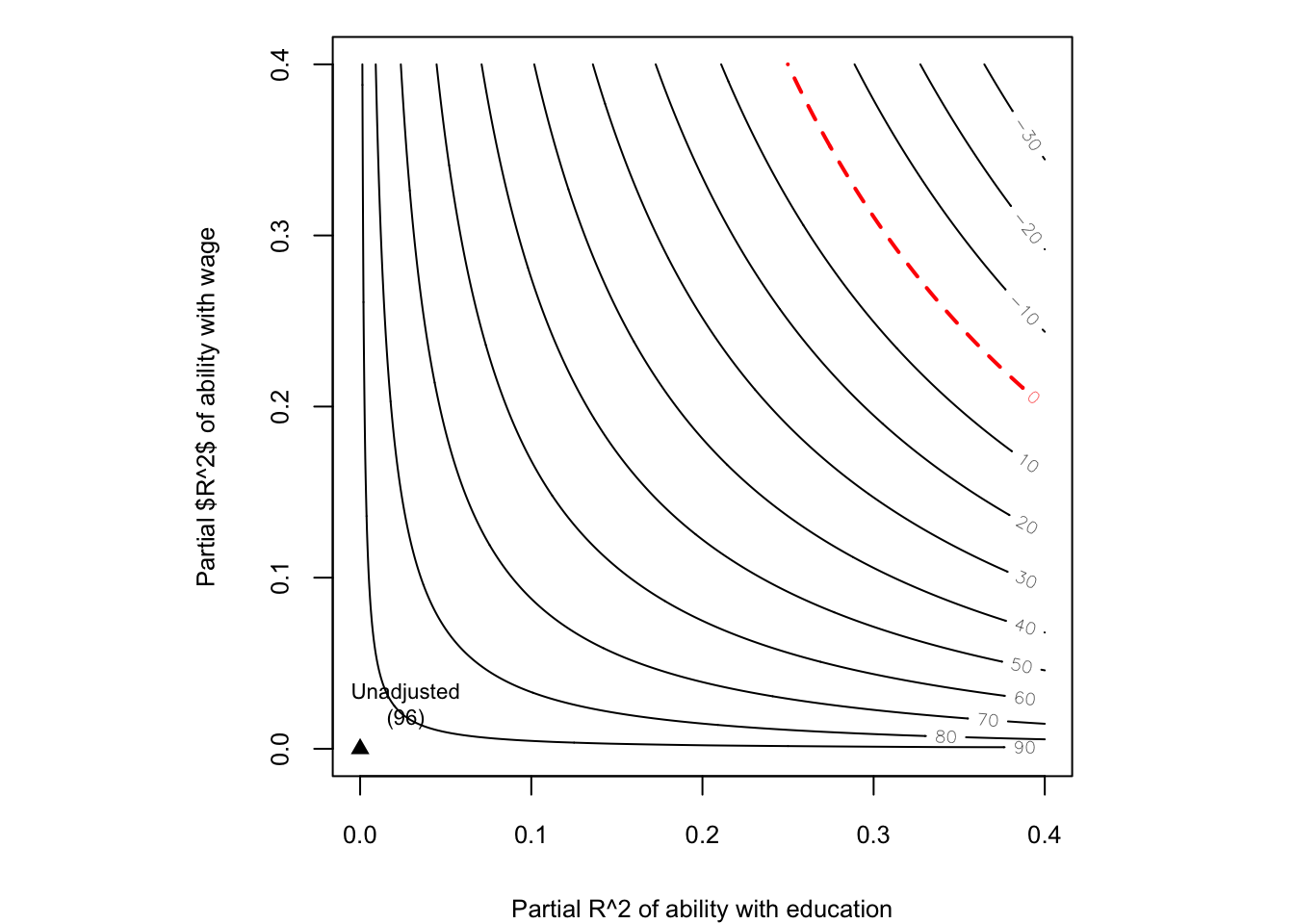

그래프를 보면 Unadjusted는 관찰되지 않은 교란요인(ability)가 영향을 주지 않을 때를 의미합니다. 즉, 회귀분석 결과와 동일합니다. 우측 상단으로 갈수록 관찰되지 않은 교란요인의 효과가 증가하고, 빨간색 dot line에 도달했을 때, ${\hat{β}}_{e d u c a t i o n} = 0$ 이 됩니다.

그래프를 보면 빨간색 dot line 위에 있는 값으로 $R_{Y \sim Z | D, X}^{2} = 0.3$ , $R_{D \sim Z | X}^{2} = 0.3$ 정도로 생각해볼 수 있습니다. 논문에서 유도한 공식을 이용해서 bias 추정치를 구해보고 확인해보겠습니다.

논문에서 partial $R^{2}$ 를 이용해서 유도한 bias 추정치는 다음과 같습니다.

$| \hat{b i a s} | = \sqrt{\frac{R_{Y \sim Z | D, X}^{2} \cdot R_{D \sim Z | X}^{2}}{1 - R_{D \sim Z | X}^{2}}} \cdot \frac{s d (Y^{⊥ X, D})}{s d (D^{⊥ X})}$

R_YZ = 0.3
R_DZ = 0.3 

DperpX <- lm(education ~ age + gender, df)$residuals
YperpXD <- lm(wage ~ ., df)$residuals

bias <- sqrt((R_YZ*R_DZ/(1 - R_DZ)))*(sd(YperpXD)/sd(DperpX))

95.94 - bias

[1] 1.697537

${\hat{β}}_{e d u c a t i o n} = 95.94$ 이고, $| \hat{b i a s} | = 94.24$ 이므로, 대략 $0$ 에 가까운 것을 확인할 수 있습니다.

Sensitivity contour plot using benchmark covariates

sensitivity contour plot을 봤을 때, 관찰되지 않은 교란요인의 treatment와 outcome에 미치는 영향에 따른 bias 효과를 확인해볼 수 있지만, 실제로 이 bias가 큰지 혹은 작은지는 주관적인 판단에 의존합니다. 즉, 이전 예시에서 $R_{Y \sim Z | D, X}^{2} = 0.3$ , $R_{D \sim Z | X}^{2} = 0.3$ 일 때, 추정된 회귀계수는 $0$ 이 되지만, $R_{Y \sim Z | D, X}^{2} = 0.3$ , $R_{D \sim Z | X}^{2} = 0.3$ 값이 큰지 혹은 작은지의 기준은 알 수 없습니다.

이러한 기준 설정의 어려움을 극복하기 위해서 관찰된 설명변수를 벤치마크하여 관찰되지 않은 교란요인이 미치는 영향의 크기를 대략적으로 추측합니다.

$\begin{array}{r} k_{D} := \frac{R_{D \sim Z | X_{- j}}^{2}}{R_{D \sim X_{j} | X_{- j}}^{2}}, k_{Y} := \frac{R_{Y \sim Z | X_{- j}, D}^{2}}{R_{Y \sim X_{j} | X_{- j}, D}^{2}} \end{array}$ $k_{D} \geq 1$ 일 때, $R_{D \sim Z | X_{- j}}^{2} \geq R_{D \sim X_{j} | X_{- j}}^{2}$ 이므로 관찰되지 않은 교란요인이 사전에 지정한 설명변수 대비 Treatment에 미치는 영향이 크다는 의미로 볼 수 있습니다. $k_{Y} \geq 1$ 일 때도 마찬가지로 관찰되지 않은 교란요인이 사전에 지정한 설명변수 대비 반응변수에 미치는 영향이 크다는 의미로 볼 수 있습니다.

sens2 <- sensemakr(model = fit, treatment = "education", 
                  benchmark_covariates = "age", 
                  kd = c(0.5, 1, 2), 
                  ky = c(0.5, 1, 2))

plot(sens2)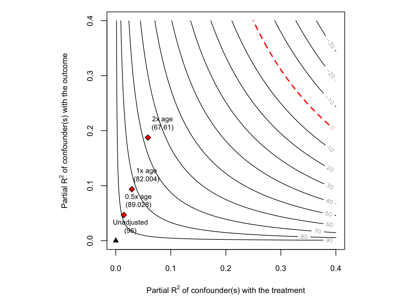

sensemakr() 함수에는 benchmark_covariates 옵션이 존재하며, $k_{D}$ , $k_{Y}$ 의 크기를 사전에 지정할 수 있습니다. 그래프를 해석해보면 관찰되지 않은 교란요인(ability)가 age의 두 배 정도의 설명력을 갖더라도, ${\hat{β}}_{e d u c a t i o n} = 67.61$ 로 값의 변화는 있지만 부호는 여전히 positive인 것을 볼 수 있습니다.

옵션을 추가할 경우 해당 plot에서 통계적 유의성 또한 체크해볼 수 있습니다.

plot(sens2, sensitivity.of = "t-value")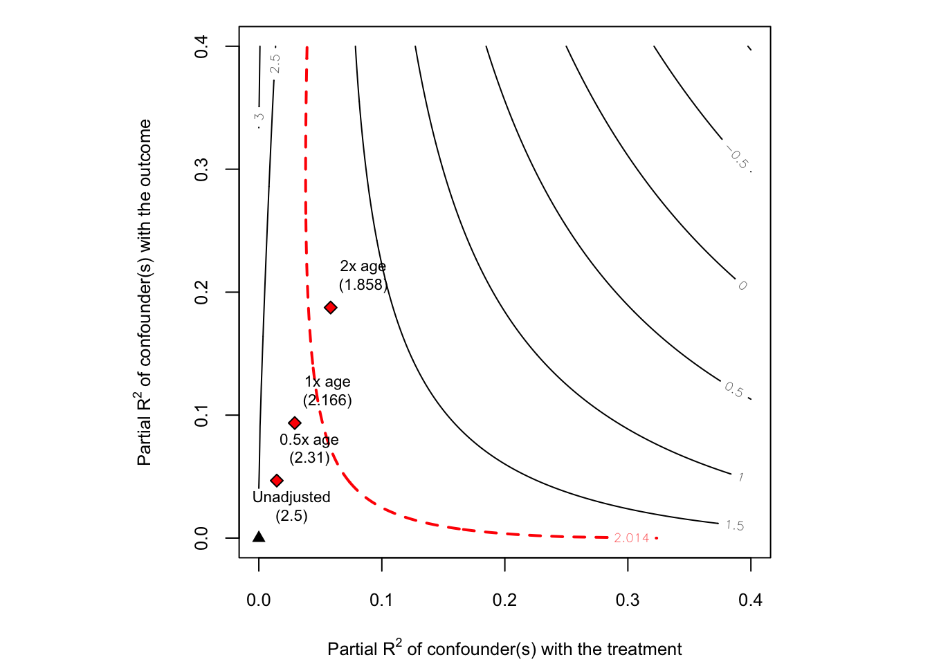

통계적 유의성을 보면 관찰되지 않은 교란요인(ability)가 $1 \times a g e$ 보다 약간 큰 정도의 설명력을 갖는다면, ${\hat{β}}_{e d u c a t i o n}$ 이 통계적으로 유의하지 않게 바뀔 수 있다는 것을 의미합니다.

plot(sens2)
add_bound_to_contour(r2dz.x = 0.3, 
                     r2yz.dx = 0.3, 
                     bound_label = "Something related to\nboth outcome and treatment")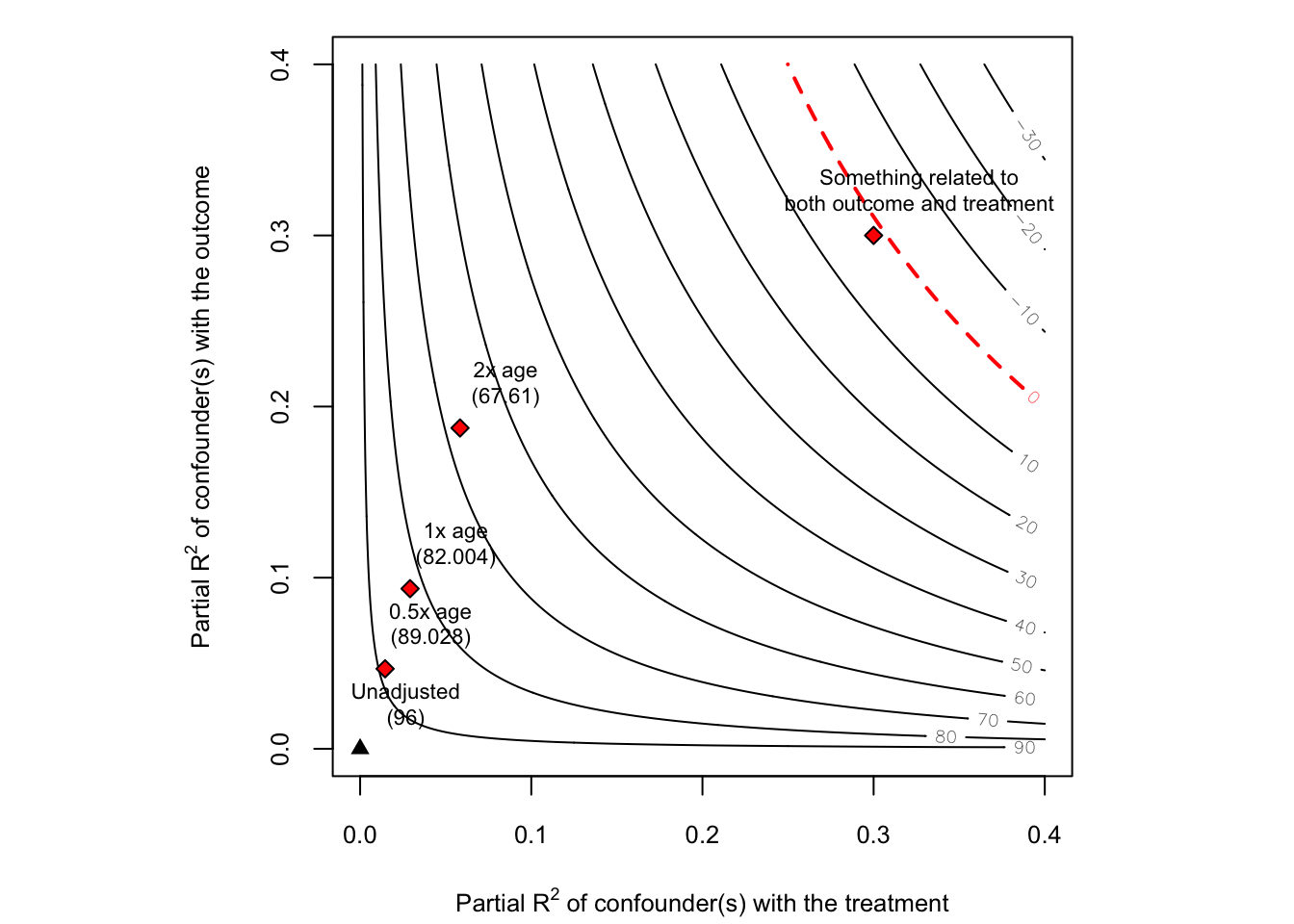

추가적으로 임의로 partial $R^{2}$ 를 설정해서 점을 찍어볼 수도 있습니다.

Sensitivity plots of extreme scenarios

extreme scenario는 outcome의 거의 모든 잔차 변동을 관찰되지 않은 교란요인이 설명한다는 의미로, $R_{Y \sim Z | D, X} = 1$ 을 의미합니다(옵션으로 $0.75, 0.5$ 일 때도 함께 제시됨). 그래프를 활용하여 extreme scenario일 때, $R_{D \sim Z | X}^{2}$ 의 변화에 따라 추정된 회귀계수가 어떻게 바뀌는지를 시각화해볼 수 있습니다.

sens3 <- sensemakr(model = fit, treatment = "education", 
                  benchmark_covariates = "age", 
                  kd = c(1, 2, 3, 4), 
                  ky = c(1, 2, 3, 4))
plot(sens3, type = "extreme", lim = 0.5)
result <- plot(sens3, type = "extreme", lim = 0.5)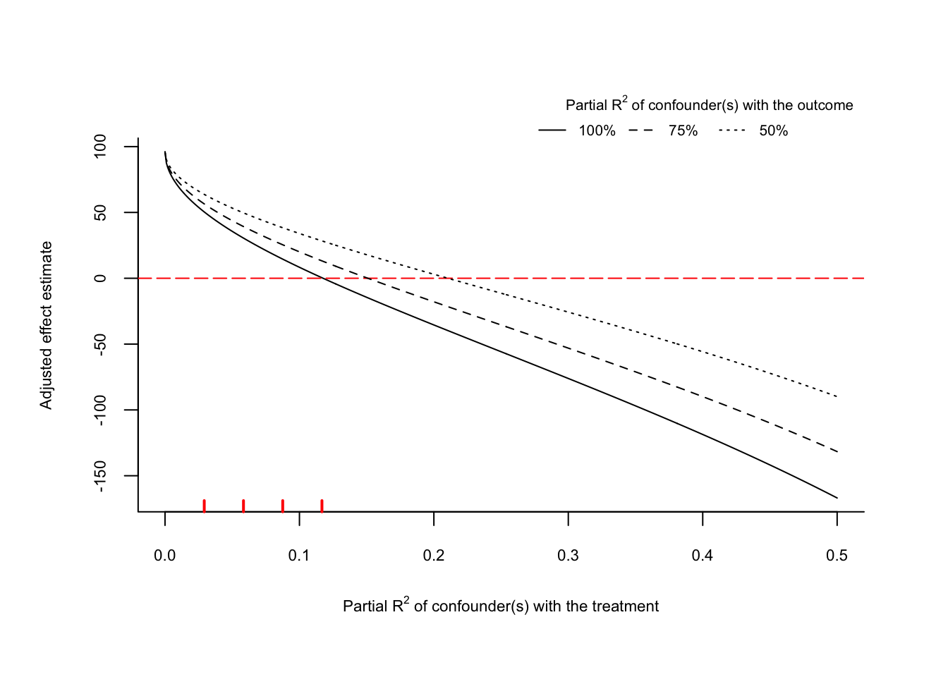

result$scenario_r2yz.dx_1[117:119,]

    r2dz.x r2yz.dx adjusted_estimate
117  0.116       1         0.7348541
118  0.117       1         0.2712232
119  0.118       1        -0.1912156

x axis : $R_{D \sim Z | X}^{2}$
y axis : $\hat{τ} = {\hat{τ}}_{r e s} - \hat{b i a s}$
line : $R_{Y \sim Z | D, X}^{2}$

그래프를 보면 빨간색 dot line은 추정된 회귀계수가 0이 되는 경우에 해당합니다. solid line은 $R_{Y \sim Z | D, X}^{2} = 1$ 일 때에 해당합니다. $R_{Y \sim Z | D, X}^{2} = 1$ 일 때, 추정된 회귀계수가 0이 되기 위해서는 $R_{D \sim Z | X}^{2} \approx 0.117$ 정도 되어야 하는 것을 확인할 수 있습니다.

또한 왼쪽 하단에 빨간색 vertical line은 benchmark로 설정한 변수에 비해 confounder가 몇 배 더 강력한지를 나타내는 것으로 kd = c(0.5, 1, 2) 옵션에서 설정한 것과 같습니다.

관찰된 설명변수 age가 education에 미치는 효과에 비해서 관찰되지 않은 교란요인이 education에 미치는 효과가 네 배정도 클 때, ${\hat{β}}_{e d u c a t i o n} \approx 0$ 이 되는 것을 확인할 수 있습니다.

상식적으로 교육기간과 나이는 충분한 양의 상관관계가 존재한다고 생각할 수 있습니다. 따라서 관찰된 설명변수 age가 education에 미치는 효과에 비해서 관찰되지 않은 교란요인이 education에 미치는 효과가 네 배정도 클 때, ${\hat{β}}_{e d u c a t i o n} \approx 0$ 이 된다는 의미는 ATE 추정량이 충분히 신뢰할 수 있고, 관찰되지 않은 교란요인에 강건하다는 것을 의미한다고 볼 수 있습니다(주관적인 해석).

dowhy tutorial

Sys.setenv(RETICULATE_PYTHON="/Users/sangdon/pytorch-test/env/bin/python")
reticulate::use_condaenv(condaenv = 'env')

import dowhy
from dowhy import CausalModel
import pandas as pd
import numpy as np
import dowhy.datasets
import os
from dowhy import CausalModel
import graphviz

from dowhy.causal_refuter import CausalRefutation
from dowhy.causal_refuter import CausalRefuter

#os.getcwd()
dat = pd.read_csv("posts/2023-02-07-sensitivity-analysis/ex_data.csv", index_col = 0)
dat.head()

dot = graphviz.Digraph() 

dot.node('age', 'age')  
dot.node('gender', 'gender')
dot.node('education', 'education')
dot.node('wage', 'wage')

dot.edge('education', 'wage')
dot.edge('gender', 'wage')
dot.edge('age', 'wage')

print(dot.source)
#dot.view()
#dot.source.replace("\t", ' ').replace("\n", ' ')

gdot = """graph[directed 1 node[id "age" label "age"]
                    node[id "gender" label "gender"]
                    node[id "education" label "education"]
                    node[id "wage" label "wage"]
                    
                    edge[source "education" target "wage"]
                    edge[source "gender" target "wage"]
                    edge[source "age" target "wage"]]"""

model = CausalModel(
            data = dat,
            treatment="education",
            outcome="wage", 
            graph = gdot
        )
        
model.view_model()

identified_estimand = model.identify_effect(proceed_when_unidentifiable=True)
print(identified_estimand)

estimate = model.estimate_effect(identified_estimand, method_name="backdoor.linear_regression")
print(estimate)

refute = model.refute_estimate(identified_estimand, 
                               estimate,
                               method_name = "add_unobserved_common_cause",
                               simulated_method_name = "linear-partial-R2",
                               benchmark_common_causes = "age",
                               effect_fraction_on_treatment = [1,2,3]
                              )

참고 자료

omitted variable bias : https://matteocourthoud.github.io/post/ovb/

unobserved confounding example : https://evalf21.classes.andrewheiss.com/example/confounding-sensitivity

R tutorial : https://cran.r-project.org/web/packages/sensemakr/vignettes/sensemakr.html

dowhy : https://www.pywhy.org/dowhy/v0.8/example_notebooks/sensitivity_analysis_testing.html?highlight=sensitivity

Citation

BibTeX citation:

@online{don2023,
  author = {Don, Don and Don, Don},
  title = {Sensitivity Analysis},
  date = {2023-02-20},
  url = {https://dondonkim.netlify.app/posts/2023-02-07-sensitivity-analysis/sensitivity.html},
  langid = {en}
}

For attribution, please cite this work as:

Don, Don, and Don Don. 2023. “Sensitivity Analysis.” February 20, 2023. https://dondonkim.netlify.app/posts/2023-02-07-sensitivity-analysis/sensitivity.html.