sensemakr

library(tidyverse)
library(sensemakr)
library(broom)

Making Sense of Sensitivity: Extending Omitted Variable Bias

Introduction

sensitivity analysis이란

• 관측 데이터로 인과추론을 하는 전략은 관측되지 않은 교란 요인(confounder)이 없다는 검증할 수 없는 가정 하에서 관측된 공변량을 조정하는 것

• 일반적으로 이러한 가정은 만족될 수 없음

• 관찰되지 않은 교란 요인이 없다는 가정이 위반되었을 때, 인과 추론에 미치는 영향을 정량적으로 확인할 수 있는 도구가 필요함

• 이는 민감도 분석(sensitivity analysis)을 통해 할 수 있음

• 이 논문에서는 다중회귀분석에 대한 sensitivity analysis만 다룸

주요 기여 사항

• OVB framework를 이용해서 다중회귀분석에서 sensitivity analysis를 효과적으로 수행하는 framework를 제시함

• unobserved confounder에 대한 분포 가정 x, treatment assignment에 대한 함수 형태 가정 x, 하에서 sensitivity analysis를 효과적으로 수행할 수 있는 tool을 개발함

• multiple confounder에 대한 sensitivity 평가도 동시에 수행 가능

개발된 tools

1. Robustness Value : unobserved confounder에 대한 coefficient의 robustness 측정

   • treatment, outcome에 대한 confounder의 연관성이 모두 RV보다 작다고 가정되는 경우 이러한 confounder는 관찰된 효과를 “설명할 수” 없음

2. $R_{Y\sim D|X}^2$ : treatment에 의해 설명되는 outcome의 변동

   • outcome에 대한 잔차의 분산을 100% 설명하는 counfounders($R_{Z\sim Y}^2=1$가 outcome에 대한 treatment의 연관성($D\sim Y$)을 제거하기 위해 treatment와 연관되어야 하는 정도($Z\sim D$)를 나타냄

3. contour plot : OVB framework를 활용한 contour plot 개발

   • 점추정치 뿐만 아니라 추론의 결과를 변경하는 confounder의 효과를 검토해볼 수 있음

4. extreme scenario : outcome에 대한 설명할 수 없는 변동이 모두 confounder일 것이라고 가정

   • confounder가 추론 결과에 문제가 되기 위해서는 treatment와 얼마나 관련이 있어야 하는지 contour plot을 통해 확인

Running example

• Research question : 집단 학살로 인한 신체적 상해를 입었을 때, 평화에 대한 개인의 태도가 어떻게 바뀌는가?

• 수단 서부 dafur 지역에서 2003 ~ 2004 약 1년간 집단 학살이 발생함

• 공격은 특정 대상이 아닌 무차별적으로 이뤄졌고, 남성과 여성 모두 중상을 입거나 사망함

• 예외 사항으로 여성의 경우 성폭행에 심하게 노출됨

• 이에 따라 평화에 대한 개인의 태도를 측정하기 위해 회귀모형을 구축해볼 수 있음

$$peaceIndex={\hat{\tau }}_{res}DirectHarm+{\hat{\beta }}_{f,res}Female+Village{\hat{\beta }}_{v,res}+X{\hat{\beta }}_{res}+{\widehat{ϵ}}_{res}$$

-   peaceIndex : 평화에 대한 개인의 태도를 측정한 index

-   DirectHarm : 공격에 의해 부상을 입거나 불구가 되었는지에 대한 dummy variable

-   female : 여성인지에 대한 이진변수

-   Village : 응답자가 속한 마을(486개의 마을이 존재함)

-   $X$ : 연령, 직업, 가구 규모 및 과거에 투표했는지 여부, 기타 등 포함된 matrix

darfur.model <- lm(peacefactor ~ directlyharmed  + village +  female +
                     age + farmer_dar + herder_dar + pastvoted + hhsize_darfur, data = darfur)

tidy(darfur.model)

# A tibble: 493 × 5
   term             estimate std.error statistic   p.value
   <chr>               <dbl>     <dbl>     <dbl>     <dbl>
 1 (Intercept)        1.08      0.315     3.44   0.000623 
 2 directlyharmed     0.0973    0.0233    4.18   0.0000318
 3 villageAbdi Dar   -0.0193    0.441    -0.0437 0.965    
 4 villageAbu Dejaj  -0.720     0.361    -1.99   0.0465   
 5 villageAbu Gamra  -0.527     0.315    -1.67   0.0948   
 6 villageAbu Gawar  -1.07      0.442    -2.41   0.0161   
 7 villageAbu Geran  -0.873     0.382    -2.29   0.0225   
 8 villageAbu Jidad  -0.488     0.383    -1.27   0.203    
 9 villageAbu Lihya  -0.571     0.348    -1.64   0.101    
10 villageAbu Mugu   -0.967     0.441    -2.19   0.0285   
# … with 483 more rows

• 분석 결과를 보면 폭력에 노출된 사람(directharmed)이 평균적으로 평화에 대해 더 친화적임($0.0973$)

• 해당 결과는 unobserved confounder가 없다는 가정 하에서 도출된 결과임

• 동료 분석가가 예를 들어 무차별적인 폭격이 이뤄졌지만, 마을 중앙에 있는 사람들이 주변에 있는 사람들에 비해 더 많은 피해를 입었을 것이라고 주장한다면?

Center 변수는 unobserved confounder로 만약 Center 변수를 추가했을 때, 회귀식을 작성하면 다음과 같음

$$peaceIndex=\hat{\tau }DirectHarm+{\hat{\beta }}_{f}Female+Village{\hat{\beta }}_v+X\hat{\beta }+\hat{\gamma }Center+{\widehat{ϵ}}_{null}$$

• Center 변수의 영향으로 ${\hat{\tau }}_{res}$와 $\hat{\tau }$는 차이가 있을 수 있음(얼마나 차이가 있는지?)

• Center 뿐만 아니라 정치적 성향, 재산 등 다양한 unobserved confounder가 존재하고, unobserved confounder 간에 상호작용 관계도 존재할 수 있음

Sensitivity in an OVB framework

The traditional Omitted variable bias

연구자가 바라는 회귀식은 unobserved confounder $Z$를 포함한 아래와 같은 식임

• $D$ : treatment variable

• $X$ : observed covariates

• $Z$ : unobserved covariates

• $Y$ : outcome variable

$$\begin{array}{r}Y=\hat{\tau }D+X\hat{\beta }+\hat{\gamma }Z+{\widehat{ϵ}}_{null}\end{array}$$

하지만 실제 회귀 식은 $Z$가 존재하지 않는 아래와 같은 식임

$$\begin{array}{r}Y={\hat{\tau }}_{res}D+X{\hat{\beta }}_{res}+{\widehat{ϵ}}_{res}\end{array}$$

따라서 $Z$의 영향으로 $\hat{\tau }$와 ${\hat{\tau }}_{res}$ 사이에 차이가 존재함

$\hat{\tau }$와 ${\hat{\tau }}_{res}$의 차이는 $\widehat{bias}$로 정의할 수 있음($\widehat{bias}={\hat{\tau }}_{res}-\hat{\tau }$)

$\widehat{bias}$을 구하기 전에 Frisch-Waugh-Lovell(FWL) thm을 이용하여 OVB solution을 구해보면 다음과 같음

1. $Y=\hat{\tau }D+X\hat{\beta }+\hat{\gamma }Z+{\widehat{ϵ}}_{null}$에 FWL을 적용하면

   1. $Y\sim X⟶Y^{\perp X}$

   2. $D\sim X⟶D^{\perp X}$

   3. $Z\sim X⟶Z^{\perp X}$

   4. $Y^{\perp X}\sim D^{\perp X}+Z^{\perp X}⟶\hat{\tau },\hat{\gamma }$

set.seed(13)
N = 10000

df <- data.frame(
    Z = rnorm(N, 1),
    X = rnorm(N, 1.5),
    D = rnorm(N, 2.5), 
    Y = rnorm(N, 3))

YperpX <- lm(Y ~ X, df)$residuals
DperpX <- lm(D ~ X, df)$residuals
ZperpX <- lm(Z ~ X, df)$residuals

resid_df <- data.frame(YperpX, DperpX, ZperpX)

print(coef(lm(YperpX ~ DperpX+ZperpX, resid_df))[c(2, 3)], digits = 2)

  DperpX   ZperpX 
-0.00072  0.01351 

print(coef(lm(Y~D+X+Z, df))[c(2, 4)], digits = 2)

       D        Z 
-0.00072  0.01351 

2. $Y={\hat{\tau }}_{res}D+X{\hat{\beta }}_{res}+{\widehat{ϵ}}_{res}$에 FWL을 적용하면

   1. $Y\sim X⟶Y^{\perp X}$

   2. $D\sim X⟶D^{\perp X}$

   3. $Y^{\perp X}\sim D^{\perp X}⟶{\hat{\tau }}_{res}$

set.seed(13)
N = 10000

df <- data.frame(
    X = rnorm(N, 1.5),
    D = rnorm(N, 2.5),
    Y = rnorm(N, 3))
YperpX <- lm(Y ~ X, df)$residuals
DperpX <- lm(D ~ X, df)$residuals
resid_df <- data.frame(YperpX, DperpX)

print(coef(lm(YperpX ~ DperpX, resid_df))[2], digits = 2)

DperpX 
0.0078 

print(coef(lm(Y~D+X, df))[2], digits = 2)

     D 
0.0078 

각 식에서 FWL을 이용해서 구한 식을 그대로 이용하면 다음과 같은 OVB solution을 도출할 수 있음

$$\begin{array}{rl}{\hat{\tau }}_{res}& =\frac{cov(D^{\perp X},Y^{\perp X})}{var(D^{\perp X})}\leftarrow Y^{\perp X}\sim D^{\perp X}\\ & =\frac{cov(D^{\perp X},\hat{\tau }{D}^{\perp X}+\hat{\gamma }{Z}^{\perp X})}{var(D^{\perp X})}\leftarrow Y^{\perp X}\sim D^{\perp X}+Z^{\perp X}\\ & =\frac{\hat{\tau }cov(D^{\perp X},D^{\perp X})+\hat{\gamma }cov(D^{\perp X},Z^{\perp X})}{var(D^{\perp X})}\\ & =\hat{\tau }+\hat{\gamma }\cdot \hat{\delta },\hat{\delta }=\frac{cov(D^{\perp X},Z^{\perp X})}{var(D^{\perp X})},\hat{\gamma }=\frac{cov(Y^{\perp X,D},Z^{\perp X,D})}{var(Z^{\perp X,D})}\end{array}$$

이를 이용해서 $\widehat{bias}$을 구하면 다음과 같이 $\hat{\gamma }$, $\hat{\delta }$로 표현할 수 있음

$$\begin{array}{r}\widehat{bias}={\hat{\tau }}_{res}-\hat{\tau }=\hat{\gamma }\cdot \hat{\delta }\end{array}$$

$\hat{\delta }(imbalance)=\frac{cov(D^{\perp X},Z^{\perp X})}{var(D^{\perp X})}$ 는 $X$를 partial out 했을 때 $Z$가 $D$에 미치는 효과로 볼 수 있음

$\hat{\gamma }(impact)=\frac{cov(Y^{\perp X,D},Z^{\perp X,D})}{var(Z^{\perp X,D})}$ 는 $X$를 partial out 했을 때 $Z$가 $Y$에 미치는 효과로 볼 수 있음

Using the traditional OVB for sensitivity analysis

• bias의 부호를 알면 추정량이 underestimate or overestimate 되었는지 알 수 있음

• $Z$는 unobserved confounder이므로 bias의 부호를 알 수 없음

• 대안으로 bias의 크기를 고려해볼 수 있음

• bias의 크기를 고려할 경우 “연구의 주요 결론에 영향을 줄 정도로 추정량을 변경하려면 unobserved confounder $Z$의 효과는 얼마나 강력해야 하는가?” 에 대해 답을 할 수 있음

• Sensitivity contour plot을 통해 확인 가능

Sensitivity contour plot

running example에 이어서 unobserved confounder인 center 변수에 대한 sensitivity contour plot을 그려보면 다음과 같음

• unadjusted : ${\hat{\tau }}_{res}$

• $x$ 축($\hat{\delta }$(imbalance)) : 마을 center에 사는 사람들의 비율 측면에서 피해를 입은 사람들이 피해를 입지 않은 사람들과 얼마나 어떻게 다른지를 나타냄

• $y$ 축($\hat{\gamma }$(impact)) : 마을 center에 사는 사람들과 마을 주변에 사는 사람들의 peaceindex가 평균적으로 어떻게 다른지를 나타냄

• 등고선 : $\hat{\tau }={\hat{\tau }}_{res}-\hat{\gamma }\cdot \hat{\delta }$

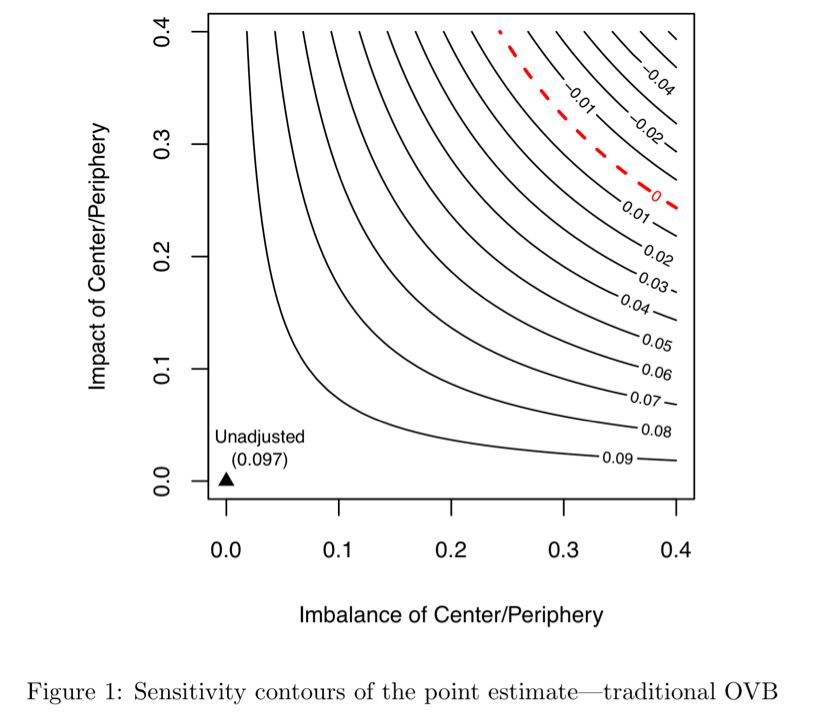
• $imbalance=25$ 일 때 : 부상을 입은 사람들은 그렇지 않은 사람들에 비해 마을 center에 살았을 확률이 25% 더 높았음을 의미함

• $imbalance=25$, $impact=0.4$ 일 때 : peaceindex에 대한 center 변수(unobserved confounder)의 영향이 DirectHarm의 영향을 $0$으로 낮추기 위해서는 약 $0.40$ 이상이어야 함을 의미함

$$\begin{array}{rl}\hat{\tau }& ={\hat{\tau }}_{res}-\hat{\gamma }\cdot \hat{\delta }\\ & =0.97-0.25\times 0.4\approx 0\end{array}$$

• 즉, contour plot을 통해 unobserved confounder가 treatment ~ outcome 관계를 없앨 정도로 강력하기 위해서는 impact와 imbalance가 어느 정도 크기여야 하는지를 확인해 볼 수 있고, 도메인 지식을 활용하여, unobserved confounder에 대한 적절한 효과를 유추해볼 수 있음
• 반면에, unobserved confounder가 center 변수 같은 이진 변수가 아니라 연속형 변수일 경우 효과의 크기를 적절하게 유추하는 것이 어려움(scale에 따라 효과의 크기가 바뀜)
• 또한, 상호작용하는 다른 많은 unobserved confounder의 효과를 고려할 수 없음
• 또한, unobserved confounder의 효과를 관찰된 변수와 벤치마킹해서 비교해볼 수 없음
• 또한, p-value, 신뢰구간의 꼴로 표현해서 해석할 수 없음
• 이러한 것을 반영하기 위해서 sensemakr 패키지 사용!

OVB with the partial $R^2$ parameterization

• $\widehat{bias}$에 대한 parameter인 $\hat{\gamma }$, $\hat{\delta }$를 partial $R^2$를 이용해서 재정의함

  • scale-free로 traditional sensitivity analysis의 문제점을 극복 가능

  • 모든 confounder들의 상호작용 효과, 비선형 효과에 대한 sensitivity를 측정할 수 있음

  • 추정치의 민감도를 평가하고, t-value, 신뢰구간을 추정할 수 있음

  • outcome의 설명되지 않은 변동의 전부 또는 대부분이 confounder로 인한 extreme scenario에 대한 sensitivity를 평가할 수 있음

  • 일상적인 보고를 쉽게 하기 위해 이러한 sensitivity 결과를 간결하게 제시하고 보다 세분화된 분석을 위한 시각적 도구를 제공

Reparameterizing the bias in terms of partial $R

• $corr(Y^{\perp X,D},Z^{\perp X,D}{)}^2=R_{Y\sim Z|X,D}^2$

• $corr(Z^{\perp X},D^{\perp X}{)}^2=R_{D\sim Z|X}^2$

• $\frac{var(Z^{\perp X,D})}{Z^{\perp X}}=1-R_{Z\sim D|X}^2$

를 이용해서 $\widehat{bias}$에 대해 reparameterizing을 하면

$$\begin{array}{rl}\widehat{bias}& =\hat{\gamma }\cdot \hat{\delta }\\ & =\sqrt{\frac{R_{Y\sim Z|D,X}^2\cdot R_{D\sim Z|X}^2}{1-R_{D\sim Z|X}^2}}\cdot \frac{sd(Y^{\perp X,D})}{sd(D^{\perp X})}\\ & =\widehat{se}({\hat{\tau }}_{res})\cdot \sqrt{\frac{R_{Y\sim Z|D,X}^2\cdot R_{D\sim Z|X}^2}{1-R_{D\sim Z|X}^2}}(df),\widehat{se}({\hat{\tau }}_{res})=\frac{sd(Y^{\perp X,D})}{sd(D^{\perp X})}\cdot \sqrt{\frac{1}{df}}\end{array}$$

Making sense of the partial $R^2$ parameterization

$$\begin{array}{rl}\text{relative bias}=\frac{\widehat{bias}}{{\hat{\tau }}_{res}}& =\frac{\widehat{se}({\hat{\tau }}_{res})}{{\hat{\tau }}_{res}}\cdot \sqrt{\frac{R_{Y\sim Z|D,X}^2\cdot R_{D\sim Z|X}^2}{1-R_{D\sim Z|X}^2}\cdot (df)}\\ & =\frac{\widehat{se}({\hat{\tau }}_{res})}{{\hat{\tau }}_{res}}\cdot R_{Y\sim Z|D,X}\cdot f_{D\sim Z|X}\cdot \sqrt{df},f_{D\sim Z|X}^2=\frac{R_{D\sim Z|X}^2}{1-R_{D\sim Z|X}^2}:\text{cohen’s f}\\ & =\frac{\sqrt{df}}{t}\cdot R_{Y\sim Z|D,X}\cdot f_{D\sim Z|X},f^2=\frac{R^2}{1-R^2}=\frac{t^2}{df}\\ & =\frac{R_{Y\sim Z|D,X}\cdot f_{D\sim Z|X}}{f_{Y\sim D|X}}\\ & =\frac{BF}{f_{Y\sim D|X}},f_{Y\sim D|X}=\frac{t_{{\hat{\tau }}_{res}}}{\sqrt{df}},BF=|R_{Y\sim Z|D,X}\cdot f_{D\sim Z|X}|\end{array}$$

relative bias의 식을 보면 분모는 treatment에 의해 설명되는 outcome의 변동이고, 기존 regression table에서 바로 구할 수 있음

분자의 경우 bias factor로 $\hat{\gamma }$, $\hat{\delta }$를 reparameterizing한 partial $R^2$로 이뤄진 항이므로, ratio를 비교해서 sensitivity를 진단해볼 수 있음

running example의 regression table에서 cohen’s f 값을 구해보면 다음과 같다.

darfur.model <- lm(peacefactor ~ directlyharmed  + village +  female +
                     age + farmer_dar + herder_dar + pastvoted + hhsize_darfur, data = darfur)

result <- tidy(darfur.model)

print(result)

# A tibble: 493 × 5
   term             estimate std.error statistic   p.value
   <chr>               <dbl>     <dbl>     <dbl>     <dbl>
 1 (Intercept)        1.08      0.315     3.44   0.000623 
 2 directlyharmed     0.0973    0.0233    4.18   0.0000318
 3 villageAbdi Dar   -0.0193    0.441    -0.0437 0.965    
 4 villageAbu Dejaj  -0.720     0.361    -1.99   0.0465   
 5 villageAbu Gamra  -0.527     0.315    -1.67   0.0948   
 6 villageAbu Gawar  -1.07      0.442    -2.41   0.0161   
 7 villageAbu Geran  -0.873     0.382    -2.29   0.0225   
 8 villageAbu Jidad  -0.488     0.383    -1.27   0.203    
 9 villageAbu Lihya  -0.571     0.348    -1.64   0.101    
10 villageAbu Mugu   -0.967     0.441    -2.19   0.0285   
# … with 483 more rows

cohen’s f

t_stat <- result %>% 
    filter(term == "directlyharmed") %>% 
    select(statistic) %>% 
    pull() %>% 
    round()

df <- glance(darfur.model)$df %>% 
    round(1)

cohen_f <- t_stat/sqrt(df)

print(cohen_f)

    numdf 
0.1803339 

• $|f|\approx 0.18$일 때, $R_{D\sim Z|X}^2=5,R_{Y\sim Z|D,X}^2=40$일 경우, $BF=0.145$ 인 것을 알 수 있음

  • $\text{relative bias}=\frac{0.145}{0.18}<1$ 이므로, directharmed coefficient는 unobserved confounder에 robust하다고 판단할 수 있음

• $|f|\approx 0.18$일 때, $R_{D\sim Z|X}^2=40,R_{Y\sim Z|D,X}^2=5$일 경우, $BF=0.183$ 인 것을 알 수 있음

  • $\text{relative bias}=\frac{0.183}{0.18}>1$ 이므로, directharmed coefficient는 unobserved confounder에 robust하지 않다고 볼 수 있음

이렇게 partial $R^2$로 reparameterizing 해서 $BF$로 표현했을 때의 장점은 unobserved confounder의 효과($Z\sim D$, $ZY$)에 대해서 symmetric하지 않다는 것임

즉, $BF=|R_{Y\sim Z|D,X}\cdot f_{D\sim Z|X}|$이므로 $BF$에서 $|R_{Y\sim Z|D,X}<1$, $f_{D\sim Z|X}<\mathrm{\infty }$로 bounding 되는 범위가 다름

이를 이용해서 extreme scenario에 대한 분석에 활용 가능?

Sensitivity statistics for routine reporting

• 전반적인 sensitivity를 쉽고 빠르게 측정하기 위한 지표로 Robust value를 고안함
• robust value는 regression table에 있는 값을 이용해서 바로 구할 수 있음
• extreme scenario를 분석하기 위해 $R_{Y\sim D}^2$를 활용함

Robustness value

• $R_{Y\sim Z|D,X}^2=R_{D\sim Z|X}^2=R{V}_q$로 가정함

$$\begin{array}{rl}{f}_q=q\cdot |f_{Y\sim D|X}|& =\sqrt{\frac{R_{Y\sim Z|D,X\cdot R_{D\sim Z|X}^2}^2}{1-R_{D\sim Z|X}^2}}\\ & =\sqrt{\frac{R{V}_q^2}{1-R{V}_q}}\end{array}$$

$$\begin{array}{r}{f}_q^2=\frac{R{V}_q^2}{1-R{V}_q}\end{array}$$

$$\begin{array}{r}{f}_q^2-f_q^2\cdot R{V}_q-R{V}_q^2=0\end{array}$$

$$\begin{array}{r}R{V}_q=\frac{1}{2}(\sqrt{f_q^4+4f_q^2}-f_q^2)\end{array}$$

• $R{V}_q\approx 1$ 경우, $Z$가 $Y$와 $D$의 거의 모든 잔차의 변동을 설명한다는 의미로 볼 수 있음

  • $R{V}_q\approx 1$ : strong confounder

• $R{V}_q\approx 0$ 경우, $Z$가 $Y$와 $D$의 일부 잔차의 변동을 설명한다는 의미로 볼 수 있음

  • $R{V}_q\approx 0$ : weak confounder

RV

tidy(darfur.model)

# A tibble: 493 × 5
   term             estimate std.error statistic   p.value
   <chr>               <dbl>     <dbl>     <dbl>     <dbl>
 1 (Intercept)        1.08      0.315     3.44   0.000623 
 2 directlyharmed     0.0973    0.0233    4.18   0.0000318
 3 villageAbdi Dar   -0.0193    0.441    -0.0437 0.965    
 4 villageAbu Dejaj  -0.720     0.361    -1.99   0.0465   
 5 villageAbu Gamra  -0.527     0.315    -1.67   0.0948   
 6 villageAbu Gawar  -1.07      0.442    -2.41   0.0161   
 7 villageAbu Geran  -0.873     0.382    -2.29   0.0225   
 8 villageAbu Jidad  -0.488     0.383    -1.27   0.203    
 9 villageAbu Lihya  -0.571     0.348    -1.64   0.101    
10 villageAbu Mugu   -0.967     0.441    -2.19   0.0285   
# … with 483 more rows

t_stat <- result %>% 
    filter(term == "directlyharmed") %>% 
    select(statistic) %>% 
    pull()

df <- glance(darfur.model)$df.residual

cohen_f <- t_stat/sqrt(df)

RV <- 1/2 * (sqrt(cohen_f^4 + 4 * cohen_f^2) - cohen_f^2)
print(RV)

[1] 0.1387764

darfur.sensitivity <- sensemakr(model = darfur.model, 
                                treatment = "directlyharmed")

darfur.sensitivity$sensitivity_stats

       treatment   estimate         se t_statistic     r2yd.x      rv_q
1 directlyharmed 0.09731582 0.02325654     4.18445 0.02187309 0.1387764
       rv_qa     f2yd.x dof
1 0.07625797 0.02236222 783

rv_q 값을 보면 결과가 같은 것을 볼 수 있음

$R_{Y\sim D}^2$ extreme scenario analysis

• $R_{Y\sim D}^2$ : $D$에 의해 유일하게 설명되는 $Y$의 변동(outcome에 대한 treatment의 효과)

  • extreme scenario case : $R_{Z\sim Y}^2=1$일 때

• extreme confounder가 outcome의 모든 잔차의 변동을 설명한다면 outcome에 대한 treatment의 효과를 제거하기 위해 treatment와 얼마나 강하게 연관되어야 하는가?

relative bias의 식을 다시 상기해보면 다음과 같음

$$\begin{array}{r}\text{relative bias}=\frac{\widehat{bias}}{{\hat{\tau }}_{res}}=\frac{R_{Y\sim Z|D,X}\times f_{D\sim Z|X}}{f_{Y\sim D|X}},f=\frac{R^2}{1-R^2}\end{array}$$

extreme scenario case($R_{Z\sim Y}^2=1$)일 때, $\text{relative bias}=1$이 되기 위해서는 $R_{D\sim Z|X}^2=R_{Y\sim D|X}^2$여야 함

이를 활용하여, extreame scenario analysis에 활용해볼 수 있음

$$\begin{array}{r}\frac{\widehat{bias}}{{\hat{\tau }}_{res}}=\frac{1\times f_{D\sim Z|X}}{|f_{Y\sim D|X}|}=1,\iff f_{D\sim Z|X}=f_{Y\sim D|X}\iff R_{D\sim Z|X}^2=R_{Y\sim D|X}^2\end{array}$$

해석

darfur.sensitivity <- sensemakr(model = darfur.model, 
                                treatment = "directlyharmed")

summary(darfur.sensitivity)

Sensitivity Analysis to Unobserved Confounding

Model Formula: peacefactor ~ directlyharmed + village + female + age + farmer_dar + 
    herder_dar + pastvoted + hhsize_darfur

Null hypothesis: q = 1 and reduce = TRUE 
-- This means we are considering biases that reduce the absolute value of the current estimate.
-- The null hypothesis deemed problematic is H0:tau = 0 

Unadjusted Estimates of 'directlyharmed': 
  Coef. estimate: 0.0973 
  Standard Error: 0.0233 
  t-value (H0:tau = 0): 4.1844 

Sensitivity Statistics:
  Partial R2 of treatment with outcome: 0.0219 
  Robustness Value, q = 1: 0.1388 
  Robustness Value, q = 1, alpha = 0.05: 0.0763 

Verbal interpretation of sensitivity statistics:

-- Partial R2 of the treatment with the outcome: an extreme confounder (orthogonal to the covariates) that explains 100% of the residual variance of the outcome, would need to explain at least 2.19% of the residual variance of the treatment to fully account for the observed estimated effect.

-- Robustness Value, q = 1: unobserved confounders (orthogonal to the covariates) that explain more than 13.88% of the residual variance of both the treatment and the outcome are strong enough to bring the point estimate to 0 (a bias of 100% of the original estimate). Conversely, unobserved confounders that do not explain more than 13.88% of the residual variance of both the treatment and the outcome are not strong enough to bring the point estimate to 0.

-- Robustness Value, q = 1, alpha = 0.05: unobserved confounders (orthogonal to the covariates) that explain more than 7.63% of the residual variance of both the treatment and the outcome are strong enough to bring the estimate to a range where it is no longer 'statistically different' from 0 (a bias of 100% of the original estimate), at the significance level of alpha = 0.05. Conversely, unobserved confounders that do not explain more than 7.63% of the residual variance of both the treatment and the outcome are not strong enough to bring the estimate to a range where it is no longer 'statistically different' from 0, at the significance level of alpha = 0.05.

Example

library(tidyverse)
df <- read.csv("ex_data.csv")[, -1]

df %>% head()

  age gender education wage
1  62   male         6 3800
2  44   male         8 4500
3  63   male         8 4700
4  33   male         7 3500
5  57 female         6 4000
6  59   male         9 3900

df$gender <- as.factor(df$gender)

fit <- lm(wage ~ ., df)
summary(fit)

Call:
lm(formula = wage ~ ., data = df)

Residuals:
    Min      1Q  Median      3Q     Max 
-958.27 -194.90   -1.32  256.00  967.54 

Coefficients:
            Estimate Std. Error t value Pr(>|t|)    
(Intercept)  2657.89     445.00   5.973 3.18e-07 ***
age            12.31       6.11   2.015   0.0498 *  
gendermale    335.11     132.69   2.526   0.0151 *  
education      95.94      38.75   2.476   0.0170 *  
---
Signif. codes:  0 '***' 0.001 '**' 0.01 '*' 0.05 '.' 0.1 ' ' 1

Residual standard error: 455.1 on 46 degrees of freedom
Multiple R-squared:  0.2549,    Adjusted R-squared:  0.2063 
F-statistic: 5.246 on 3 and 46 DF,  p-value: 0.003379

• education의 coef는 양수임

• unobserved confounder(ability)가 있으므로, OVB가 존재함

library(sensemakr)
sens <- sensemakr(model = fit, treatment = "education")
sens

Sensitivity Analysis to Unobserved Confounding

Model Formula: wage ~ age + gender + education

Null hypothesis: q = 1 and reduce = TRUE 

Unadjusted Estimates of ' education ':
  Coef. estimate: 95.94369 
  Standard Error: 38.75212 
  t-value: 2.47583 

Sensitivity Statistics:
  Partial R2 of treatment with outcome: 0.11759 
  Robustness Value, q = 1 : 0.30444 
  Robustness Value, q = 1 alpha = 0.05 : 0.06273 

For more information, check summary.

• 교육이 임금에 미치는 영향의 부호가 바뀌려면, 교육과 임금의 residual variance 중 어느 정도를 ability로 설명해야 하는지?

summary(sens)

Sensitivity Analysis to Unobserved Confounding

Model Formula: wage ~ age + gender + education

Null hypothesis: q = 1 and reduce = TRUE 
-- This means we are considering biases that reduce the absolute value of the current estimate.
-- The null hypothesis deemed problematic is H0:tau = 0 

Unadjusted Estimates of 'education': 
  Coef. estimate: 95.9437 
  Standard Error: 38.7521 
  t-value (H0:tau = 0): 2.4758 

Sensitivity Statistics:
  Partial R2 of treatment with outcome: 0.1176 
  Robustness Value, q = 1: 0.3044 
  Robustness Value, q = 1, alpha = 0.05: 0.0627 

Verbal interpretation of sensitivity statistics:

-- Partial R2 of the treatment with the outcome: an extreme confounder (orthogonal to the covariates) that explains 100% of the residual variance of the outcome, would need to explain at least 11.76% of the residual variance of the treatment to fully account for the observed estimated effect.

-- Robustness Value, q = 1: unobserved confounders (orthogonal to the covariates) that explain more than 30.44% of the residual variance of both the treatment and the outcome are strong enough to bring the point estimate to 0 (a bias of 100% of the original estimate). Conversely, unobserved confounders that do not explain more than 30.44% of the residual variance of both the treatment and the outcome are not strong enough to bring the point estimate to 0.

-- Robustness Value, q = 1, alpha = 0.05: unobserved confounders (orthogonal to the covariates) that explain more than 6.27% of the residual variance of both the treatment and the outcome are strong enough to bring the estimate to a range where it is no longer 'statistically different' from 0 (a bias of 100% of the original estimate), at the significance level of alpha = 0.05. Conversely, unobserved confounders that do not explain more than 6.27% of the residual variance of both the treatment and the outcome are not strong enough to bring the estimate to a range where it is no longer 'statistically different' from 0, at the significance level of alpha = 0.05.

plot(sens, xlab = "Partial R^2 of ability with education", 
     ylab = "Partial $R^2$ of ability with wage")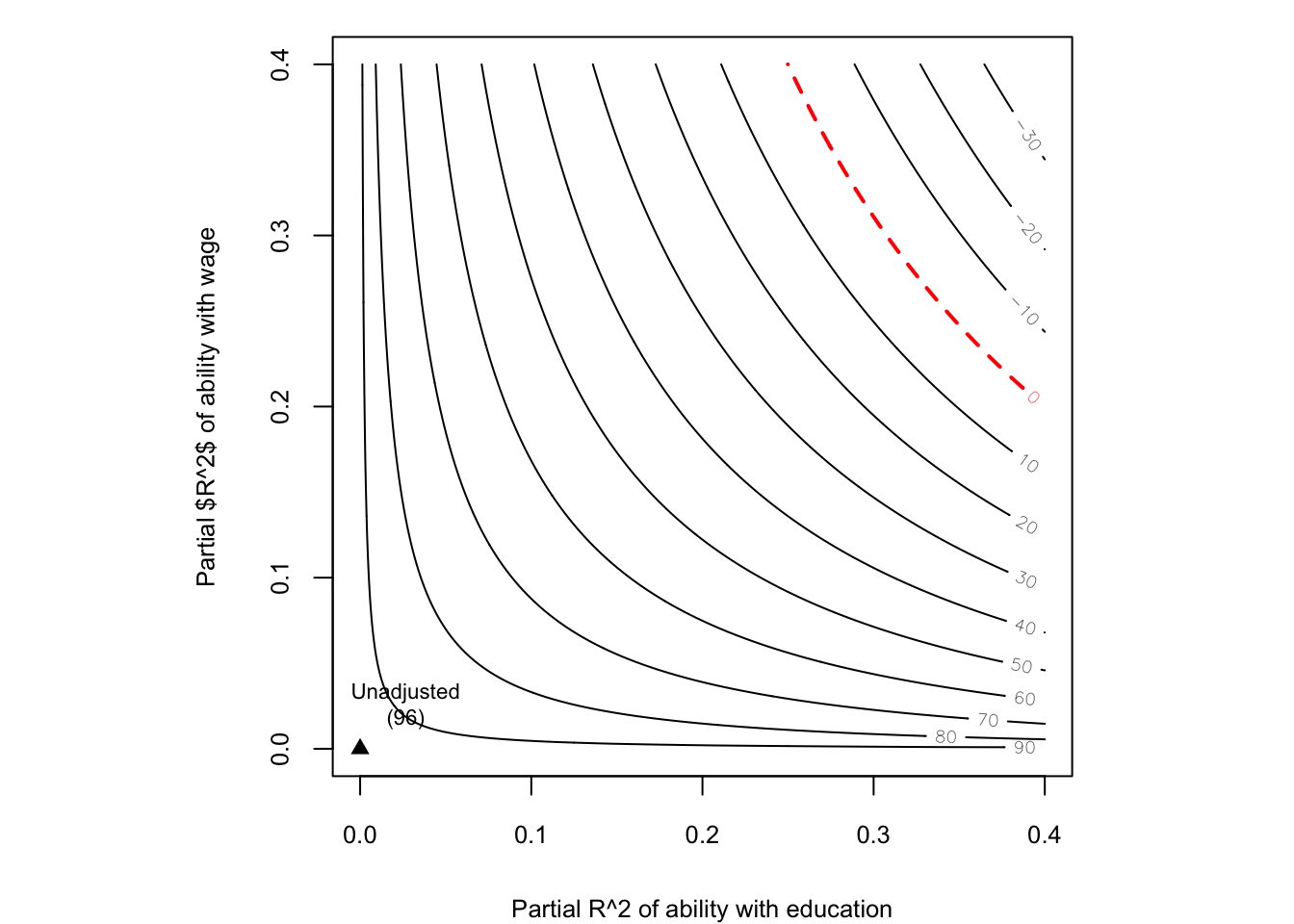

• unadjusted는 unobserved confounder인 ability가 wage, education에 미치는 효과가 없을 때를 의미함

  • 위에서 lm 결과와 동일함

• 우측 상단으로 갈수록 ability의 power는 증가하고, 추정된 회귀계수 값은 감소함

• 빨간 점선일 때, 추정된 회귀계수 값은 0이 됨

sens2 <- sensemakr(model = fit, treatment = "education", 
                  benchmark_covariates = "age", 
                  kd = c(0.5, 1, 2), 
                  ky = c(0.5, 1, 2))

plot(sens2)

plot(sens, type = "extreme")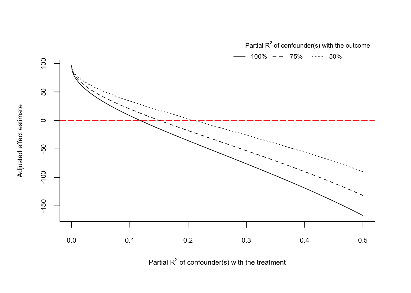

참고자료

https://bookdown.org/ts_robinson1994/10_fundamental_theorems_for_econometrics/frisch.html

https://arelbundock.com/posts/robustness_values/

https://web.stanford.edu/~mrosenfe/soc_meth_proj3/matrix_OLS_2_Beck_UCSD.pdf

https://py-why.github.io/dowhy/v0.8/example_notebooks/sensitivity_analysis_testing.html?highlight=sensitivity

Citation

BibTeX citation:

@online{don2022,
  author = {Don, Don and Don, Don},
  title = {Sensemakr},
  date = {2022-06-24},
  url = {https://dondonkim.netlify.app/posts/sensmakr/sensmakr.html},
  langid = {en}
}

For attribution, please cite this work as:

Don, Don, and Don Don. 2022. “Sensemakr.” June 24, 2022. https://dondonkim.netlify.app/posts/sensmakr/sensmakr.html.